Python : 非線形方程式の解法
はじめに
Pythonista は,iOS 用 Python 2.7 のプログラミング環境であり,numpy および matplotlib が同梱されており,大変便利なものですが,scipy を使うことができません.
よって,非線形方程式を解くには,基本に立ち戻ってコーディングしてやる必要があります.
これに対し,OS X や Windows 用 Python(私の場合は Python 3.4)では,scipy を使うことができるため,非線形方程式を scipy の機能を用いて簡単なコーディングにより解くことができます.
ここでは,Pythonista (scipy 無し) と Python + scipy による非線形方程式の解法の事例を紹介します.
なお,コーディングが簡単というだけであり,当然のことながら,scipyを用いた場合でも,初期値によっては必ずしも望むべき領域にある解が得られるとは限らないことには,注意が必要です.
Pythonista (iOS Python 2.7)での二分法
以下のプログラムは,越流堰において,流量$Q$が与えられた時の越流水深$x$を二分法により求めるものです.
解くべき方程式は,以下のとおり.$B$および$C$は定数,$Q$は既知であり,$x$が求めるべき越流水深です.
$$
Q-C\cdot B\cdot x^{1.5}=0
$$
# coding: utf-8
from math import *

def func(x,Q):
    B=19.0
    W=2.453
    C=1.28+1.42*x/W
    return Q-C*B*x**(1.5)

def cal(x01,y02,Q):
    imax=100
    eps=1.0e-6
    x1=x01
    x2=x02
    for i in range(0,imax):
        xi=0.5*(x1+x2)
        f1=func(x1,Q)
        f2=func(x2,Q)
        fi=func(xi,Q)
        if abs(x2-x1) < eps: break
        if f1*fi < 0.0: x2=xi
        if fi*f2 < 0.0: x1=xi
        print '{0:5d}{1:15.7e}'.format(i,xi)
    return xi

#main routine
Q=30.0
x01=0.001
x02=10.000
x=cal(x01,x02,Q)
print '{0:15.7e}'.format(x)
Pythonista (iOS Python 2.7)での Newton-Raphson法
連立非線型方程式
$$
\begin{cases}
f(x,y)=0 \\
g(x,y)=0
\end{cases}
$$
を解くには,以下の増分形連立方程式を逐次解き収束点を求めれば良い.
$$
\begin{bmatrix}
\cfrac{\partial f(x_i,y_i)}{\partial x} & \cfrac{\partial f(x_i,y_i)}{\partial y} \\
\cfrac{\partial g(x_i,y_i)}{\partial x} & \cfrac{\partial g(x_i,y_i)}{\partial y} \\
\end{bmatrix}
\begin{Bmatrix}
\Delta x \\
\Delta y
\end{Bmatrix}
=
\begin{Bmatrix}
-f(x_i,y_i) \\
-g(x_i,y_i)
\end{Bmatrix}
$$
$$
\begin{cases}
x_{i+1}=x_i+\Delta x \\
y_{i+1}=y_i+\Delta y
\end{cases}
$$
以下の事例は,2つの円の交点を求めるためのプログラムであり,関数$f$および$g$は以下のものである.
$$
\begin{cases}
f(x,y)=(x-a_1)^2+(y-b_1)^2-r_1^2=0 \\
g(x,y)=(x-a_2)^2+(y-b_2)^2-r_2^2=0
\end{cases}
$$
# coding: utf-8
from math import *

def func(x,y,a1,b1,a2,b2,r1,r2):
    f=(x-a1)**2+(y-b1)**2-r1**2
    g=(x-a2)**2+(y-b2)**2-r2**2
    fx=2*(x-a1)
    fy=2*(y-b1)
    gx=2*(x-a2)
    gy=2*(y-b2)
    return f,g,fx,fy,gx,gy

def newton(a1,b1,r1,a2,b2,r2,x0,y0):
    itmax=100
    eps=1.0e-6
    x=x0
    y=y0
    for i in range(0,itmax):
        f,g,fx,fy,gx,gy=func(x,y,a1,b1,a2,b2,r1,r2)
        coef=fx*gy-fy*gx
        dx=(-f*gy+g*fy)/coef
        dy=( f*gx-g*fx)/coef
        x=x+dx
        y=y+dy
        print '{0:5d}{1:15.7e}{2:15.7e}{3:15.7e}{4:15.7e}'.format(i,x,y,dx,dy)
        if abs(dx) < eps and abs(dy) < eps: break
    return x,y

#main routine
a1=0.000; b1= 5.000; r1=10.000
a2=0.000; b2=-5.000; r2= 3.000
x0=-5.0; y0=-0.1
x,y=newton(a1,b1,r1,a2,b2,r2,x0,y0)
print '{0:15.7e}{1:15.7e}'.format(x,y)
Scipyの利用 (Mac:Python 3.4)
Scipyを用いて,上記で扱った2つの問題を解いてみます.
# Intersection coordinates of 2 circles
#import numpy as np
from scipy import optimize

def func1(x,Q):
    B=19.0
    W=2.453
    C=1.28+1.42*x/W
    return Q-C*B*x**(1.5)

def func2(x,a1,b1,r1,a2,b2,r2):
    return [(x[0]-a1)**2+(x[1]-b1)**2-r1**2,
            (x[0]-a2)**2+(x[1]-b2)**2-r2**2]

#Main routine
#Solution of non-linear equation
Q=30.0
res=optimize.brentq(func1,0.001,10,args=(Q))
print('{0:15.7e}'.format(res))

#Solution of nonlinear simultaneous equation (2x2)
a1=0.000; b1= 5.000; r1=10.000
a2=0.000; b2=-5.000; r2= 3.000
sol=optimize.root(func2, [-5.0, -0.1], args=(a1,b1,r1,a2,b2,r2), method='broyden1')
print('{0:15.7e}{1:15.7e}'.format(sol.x[0],sol.x[1]))
Scipyによるコーディングは以下を参考にしました.
http://org-technology.com/posts/scipy-root-finding-scalar-functions.html
http://org-technology.com/posts/scipy-root-finding-multidimensional-functions.html
高速Fourier変換(FFT)
地震動のフーリエスペクトル
nimpy の fft を使っています.
import numpy as np
import matplotlib.pyplot as pl

def INPDAT():
    fnameR='dat_acc_TCGH16_EW2.csv'
    fin=open(fnameR,'r')
    text=fin.readline()
    text=fin.readline();text=text.strip();text=text.split(',');dt=float(text[1])
    text=fin.readline();text=text.strip();text=text.split(',');ndata=int(text[1])
    wave=[]
    for i in range(0,ndata):
        text=fin.readline();text=text.strip();wave=wave+[float(text)]
    fin.close()
    return dt,ndata,wave

dt,ndata,wave=INPDAT()
x=np.array(wave)
nn=2
while nn < ndata:
    nn=nn*2
xx=np.zeros(nn)
xx[0:ndata]=xx[0:ndata]+x[0:ndata]
sp=np.fft.fft(xx,nn)/nn
spa=np.sqrt(sp.real[0:int(nn/2)+1]**2+sp.imag[0:int(nn/2)+1]**2)*dt*nn
fk=np.arange(0,nn/2+1)/nn/dt

pl.xlabel('Frequency (Hz)',fontsize=12)
pl.ylabel('Fourier Spectrunm (gal*sec)',fontsize=12)
pl.xlim(0,20)
pl.ylim(0.1,10000)
pl.semilogy(fk,spa,linewidth=0.5,color='blue')
pl.grid(True,ls='-', color='0.65')
pl.show()
プログラムと入出力事例
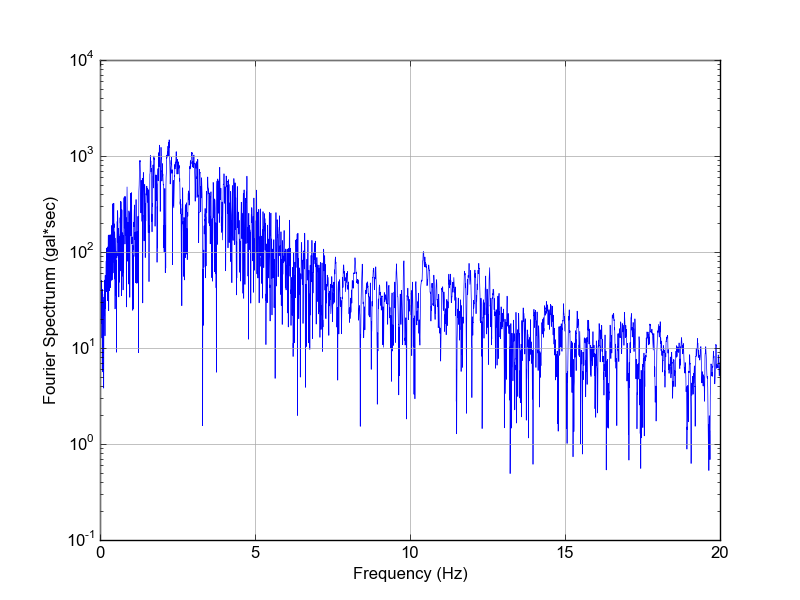 |
| fig_fft_sp.png |
|---|
numpy と scipy のFFTパック
import numpy as np
from scipy import fftpack

def FFT_N(xx):
    sp=np.fft.fft(xx)/nn
    spa=np.sqrt(sp.real**2+sp.imag**2)
    wv=np.fft.ifft(sp*nn)
    return sp,spa,wv

def FFT_S(xx):
    sp=fftpack.fft(xx)/nn
    spa=np.sqrt(sp.real**2+sp.imag**2)
    wv=fftpack.ifft(sp*nn)
    return sp,spa,wv


#x=np.array([0.998, 0.567, 0.966, 0.748, 0.367, 0.481, 0.074, 0.005,
#            0.347, 0.342, 0.218, 0.133, 0.901, 0.387, 0.445, 0.662])
x=np.random.random_sample(10)
nd=len(x)
nn=2
while nn < nd:
    nn=nn*2
xx=np.zeros(nn)
xx[0:nd]=xx[0:nd]+x[0:nd]
sp1,spa1,wv1=FFT_N(xx)
sp2,spa2,wv2=FFT_S(xx)

print('%7s %7s %7s %7s %7s %7s'\
       %('x','Re(Ck)','Im(Ck)','Abs(Ck)','Re(x)','Re(x)'))
for i in range(0,nn):
    print('%7.3f %7.3f %7.3f %7.3f %7.3f %7.3f'\
           %(xx[i],sp1.real[i],sp1.imag[i],spa1[i],wv1.real[i],wv1.imag[i]))

print('%7s %7s %7s %7s %7s %7s'\
       %('x','Re(Ck)','Im(Ck)','Abs(Ck)','Re(x)','Re(x)'))
for i in range(0,nn):
    print('%7.3f %7.3f %7.3f %7.3f %7.3f %7.3f'\
           %(xx[i],sp2.real[i],sp2.imag[i],spa2[i],wv2.real[i],wv2.imag[i]))
プログラムと入出力事例
出力は以下に示す通り.
numpy_fft
      x  Re(Ck)  Im(Ck) Abs(Ck)   Re(x)   Re(x)
  0.606   0.184   0.000   0.184   0.606  -0.000
  0.025   0.001  -0.080   0.080   0.025   0.000
  0.644   0.059  -0.008   0.060   0.644  -0.000
  0.067  -0.015  -0.035   0.038   0.067   0.000
  0.338   0.031   0.012   0.033   0.338   0.000
  0.064  -0.004   0.013   0.014   0.064  -0.000
  0.379   0.046   0.025   0.052   0.379   0.000
  0.239   0.027   0.053   0.059   0.239   0.000
  0.572   0.133   0.000   0.133   0.572   0.000
  0.017   0.027  -0.053   0.059   0.017   0.000
  0.000   0.046  -0.025   0.052   0.000   0.000
  0.000  -0.004  -0.013   0.014  -0.000  -0.000
  0.000   0.031  -0.012   0.033   0.000   0.000
  0.000  -0.015   0.035   0.038  -0.000  -0.000
  0.000   0.059   0.008   0.060   0.000  -0.000
  0.000   0.001   0.080   0.080  -0.000   0.000

scipy_fft
      x  Re(Ck)  Im(Ck) Abs(Ck)   Re(x)   Re(x)
  0.606   0.184   0.000   0.184   0.606   0.000
  0.025   0.001  -0.080   0.080   0.025   0.000
  0.644   0.059  -0.008   0.060   0.644  -0.000
  0.067  -0.015  -0.035   0.038   0.067  -0.000
  0.338   0.031   0.012   0.033   0.338   0.000
  0.064  -0.004   0.013   0.014   0.064  -0.000
  0.379   0.046   0.025   0.052   0.379  -0.000
  0.239   0.027   0.053   0.059   0.239  -0.000
  0.572   0.133   0.000   0.133   0.572   0.000
  0.017   0.027  -0.053   0.059   0.017   0.000
  0.000   0.046  -0.025   0.052  -0.000   0.000
  0.000  -0.004  -0.013   0.014  -0.000   0.000
  0.000   0.031  -0.012   0.033  -0.000   0.000
  0.000  -0.015   0.035   0.038  -0.000   0.000
  0.000   0.059   0.008   0.060  -0.000   0.000
  0.000   0.001   0.080   0.080  -0.000   0.000
3次スプライン内挿
3次スプライン内挿プログラム
scipyのスプライン内挿モジュールを用います.
一般的に使えるように,ファイル名 (fnameR),内挿値を計算する範囲と分割幅 (xmin, xmax, dx) はコマンドライン入力します.
結果は,画面に数値を出力するとともに,matplotlibを用いてグラフ化しています.ただしグラフは結果確認目的のみのため,報告書などに使えるレベルではありません.
import sys
import numpy as np
from scipy.interpolate import interp1d
import matplotlib.pyplot as plt

argv=sys.argv
fnameR=argv[1]
xmin=float(argv[2])
xmax=float(argv[3])
dx  =float(argv[4])

data1 = np.loadtxt(fnameR, usecols=(0,1))
f = interp1d(data1[:,0], data1[:,1], kind='cubic')

ndx=int((xmax-xmin)/dx)+1
xnew = np.linspace(xmin,xmax,ndx)
for i in range(0,ndx):
    print(xnew[i],f(xnew[i]))
plt.plot(data1[:,0],data1[:,1],'ro',label='Observed')
plt.plot(xnew,f(xnew),'b-',label='cubic')
plt.legend(loc='lower right')
plt.xlabel('$x$')
plt.ylabel('$y$ (python)')
plt.show()
実行用スクリプト
python3 py_eng_spline.py inp_data_spl.txt -10 -10 0.1
プログラムと入出力事例
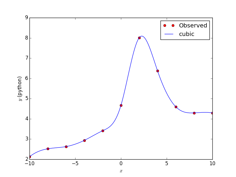 |
| fig_spl.png |
|---|