Outline of a program 'f90_fem_seep.f90'
- This is a program for 2D Steady Seepage Flow Analysis. This program can not treat unsteady problem.
- This program can do the saturated-unsaturated seepage flow analysis in the vertical section, and saturated seepage flow analysis in the horizontal and vertical section.
- Von Genuchten model is used as a unsaturated ground model.
- In this program, 3 node element or 4 node element can be used. Mixed model of 3 node elements and 4 node elements can not be solved. User of this program needs to choose either 3 node model or 4 node model.
- Linear triangular element is used as a 3 node element. 1 node has 2 degrees of freedom in horizontal direction and vertical direction.
- 4 node isoparametric element with 4 Gauss points is used as a 4 node element. 1 node has 2 degrees of freedom in horizontal direction and vertical direction.
- Thickness of the element is unit thickness and it is not changeable.
- As boundary conditions, impervious boundary, given total head boundary, given discharge boundary and saturation point boundary can be considered.
- In coordinate system, x-direction is defined as right direction and z-direction is defined as upward direction.
- Only an isotropic material can be treated.
- Nodal head must be inputted as total head and solution of simultaneous equations is described as total head.
- Pressure head is calculated as the difference between total head and position head.
- Simultaneous linear equations are solved using Cholesky method for banded matrix.
- Convergence criterion is that the case change of pressure head becomes less than 1$\times$10$^{-6}$. Upper limit of iteration is set to 100 times.
- Input/Output file name can be defined arbitrarily with the format of 'csv' and those are inputted from command line of a terminal.
- Used language for program is 'Fortran 90' and used compiler is 'GNU gfortran.'
| Workable condition | |
|---|---|
| Item | Description |
| Element | Triangle & Quadrilateral element |
| Impervious boundary | No-input means impervious boundary |
| Total head given boundary | Specify the nodes and total head of the nodes |
| Discharge given boundary | Specify the nodes and discharge. Positive value of discharge means in-flow, and negative value of discharge means out-flow from a element. |
| Satulation point boundary | Specify the nodes which have the possibility of becoming saturation point. Pressure head at these points are zero or negative value and signs of discharge are negative (out-flow) |
| Section for analysis | Choose either vertical or horizontal section. Pressure head in vertical section is given as the difference between total head and position head, and pressure head in horizontal section is the same as total head in it. |
Format of input file ('csv' format)
Comment                              # Comment
nod,NODT,NELT,MATEL,KOH,KOQ,KOU,idan # basic values for analysis
Ak0,alpha,em                         # Material properties
    ....(1 to MATEL)....             #
node-1,node-2,node-3(,node-4),matno  # Element-nodes relationship, material set number
    ....(1 to MATEL)....             #  (counterclockwise order of node numbers)
x,z,hvec                             # Node coordinate, initial value of total head
    ....(1 to NODT)....              # (x: right-direction, z: upward-direction)
nokh,Hinp                            # Node number of given total head boundary, total head of node
    ....(1 to KOH)....               # (Omit data input if KOH=0)
nokq,Qinp                            # Node number of given discharge boundary, discharge of node
    ....(1 to KOQ)....               # (Omit data input if KOQ=0)
noku                                 # Node number of saturation point
    ....(1 to KOU)....               # (Omit data input if KOU=0)
| nod | : Number of nodes of each element (3 or 4) | nokh | : Node number with given total head |
| NODT | : Number of nodes | nokq | : Node number with given discharge |
| NELT | : Number of elements | noqu | : Node number with saturation point |
| MATEL | : Number of material sets | Hinp | : Total head at specified node |
| KOH | : Number of nodes with given total head | Qinp | : Discharge at specified node |
| KOQ | : Number of nodes with given discharge | (positive: in-flow, negative: out-flow) | |
| KOU | : Number of nodes with saturation point | Ak0 | : Permeability coefficient of element (saturated) |
| idan | : Section (0: Vertical, 1: horizontal) | alpha | : Unsaturated property ($\alpha$) of element |
| matno | : Material set number | em | : Unsaturated property ($m$) of element |
Notice
- Unsaturated properties are $\alpha$ and $m$ on van Genuchten model.
\begin{align*} &S_e=\left\{\frac{1}{1+\left(\alpha\cdot h_s\right)^n}\right\}^m \qquad\qquad n=\frac{1}{1-m} \quad & (0 < m < 1) \\ &K_r=(S_e)^{0.5}\cdot\left\{1-\left(1-S_e{}^{1/m}\right)^m\right\}^2 & (0 \leqq S_r, K_r \leqq 1) \\ &K=K_r \cdot K_0 \end{align*}
$K$ : Permeability coefficient $S_e$ : Degree of saturation $K_0$ : Saturated permeability coefficient $h_s$ : Suction head $K_r$ : Relative hydraulic conductivity function $\alpha$ : Scaling parameter $m$ : Non-dimensional parameter
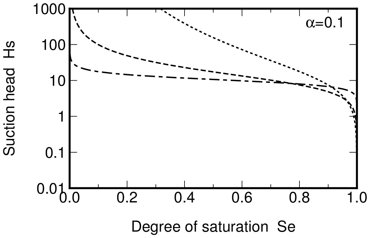
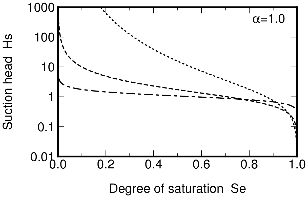
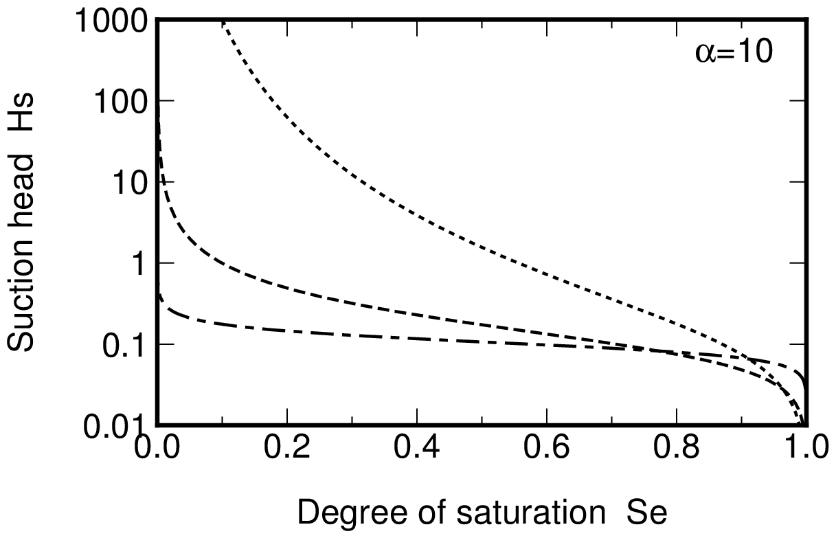
Relationship between Degree of saturation and Sunction head
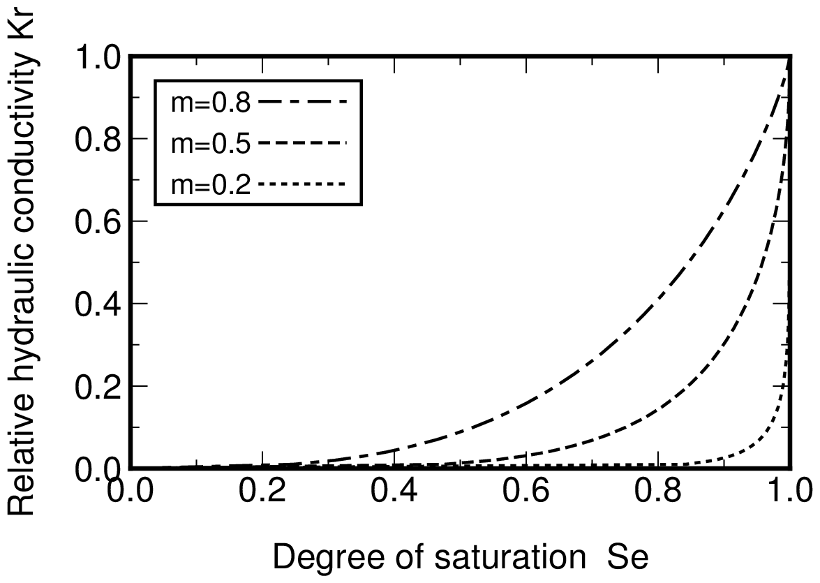
Relationship between Degree of saturation and Relative hydraulic conductivityg
- Regarding the values of $\alpha$ and $m$, Webmaster usually use $\alpha=0.1$ and $m=0.7$.
- Condition of node at which noting is inputted is no discharge. (in-flow discharge + out-flow discharge = 0) If input of in-flow or out-flow discharge is wanted especially, the values of KOQ, nokq and Qinp should be inputted.
- The discharge is known if total head is unknown at a node, and total head is known if discharge is unknown at a node. This condition is maintained except the node with saturation point.
- Nodes which have the possibility becoming saturation point such as downstream slope of embankment dam shall be specified as saturation point boundary with input of KOU and noku.
- It is necessary to input initial total heads for all nodes for iterative process of saturates-unsaturated analysis. It is better to input minimum total head in the domain. If proper initial total heads are not inputted, unsuitable results may be obtained.
Format of output file ('csv' format)
Comment
nod,NODT,NELT,MATEL,KOH,KOQ,KOU,idan
(Each value of above items)
*node characteristics
node,x,z,KOH,KOQ,KOU,Hinp,Qinp
    node : Node number
    x,z  : (x,z) Coordinate of node
    KOH  : Node with given total head (1: yes, 0: no)
    KOQ  : Node with given discharge (1: yes, 0: no)
    KOU  : Node with saturation point (1: yes, 0: no)
    Hinp : Given total head (if KOH=0, value=0)
    Qinp : Given discharge (if KOQ=0, value=0)
  .....(1 to NODT).....
*element characteristics
element,node-1,node-2,node-3(,node-4),Ak0,alpha,em,matno
    element : Element number
    node-1,node-2,node-3(,node-4) : Element-nodes relationship
    Ak0     : Permeability coefficient of element (saturated)
    alpha   : Unsaturated property $\alpha$
    em      : Unsaturated property $m$
    matno   : material set number
  .....(1 to NELT).....
*node value
node,x,z,hvec,qvec,pvec
    node : Node number
    x    : x-coordinate of node
    z    : z-coordinate of node
    hvec : Total head of node
    qvec : Discharge of node
    pvec : Pressure head of node (total head $-$ position head)
  .....(1 to NODT).....
*element value
element,xg,zg,vx,vz,vm,Ak0,Akr,matno
    element : Element number
    xg      : x-coordinate of COG of element
    zg      : z-coordinate of COG of element
    vx      : x-direction mean velocity in global coordinate system
    vz      : z-direction mean velocity in global coordinate system
    vm      : Combined mean velocity in global coordinate system
    Ak0     : Permeability coefficient (saturated)
    Akr     : Relative hydraulic conductivity function of element
    matno   : Material set number
  .....(1 to NELT).....
#,Summary
#,item,QTi,QTo
#,discharge,sum total of in-flow,sum total of out-flow
#,item,ne,vmax,xg,zg
#,vmmax,element number,max.velocity in all elements,x-coordinate of COG,,z-coordinate of COG
#,vimax,element number,max.velocity in in-flow elements,x-coordinate of COG,,z-coordinate of COG
#,vomax,element number,max.velocity in out-flow elements,x-coordinate of COG,,z-coordinate of COG
#,NELT=(Number of elements), NODT=(Number of nodes), nt=(nt), mm=(mm), ib=(ib)
#,nnn=(Number of iteration), icount=(Number of converged degrees of freedom)
#,Calculation time=(Calculation time)
#,Date_time=(date of execution)
    nt : Total degrees of freedom of FE equation
    mm : Dimension of reduced FE equation
    ib : band width of reduced FE equation
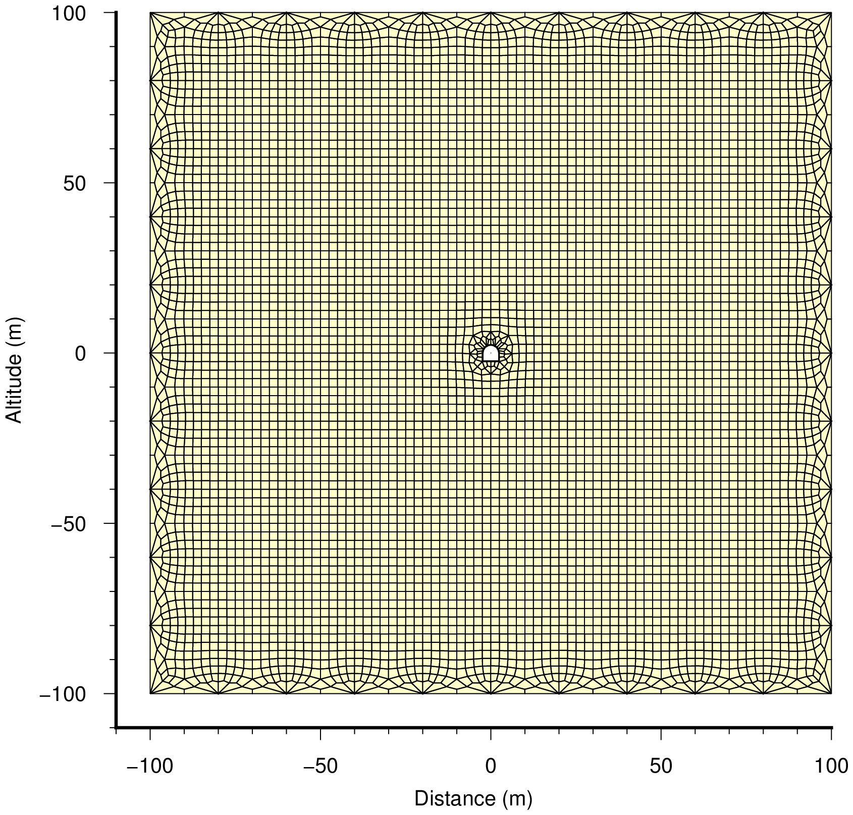
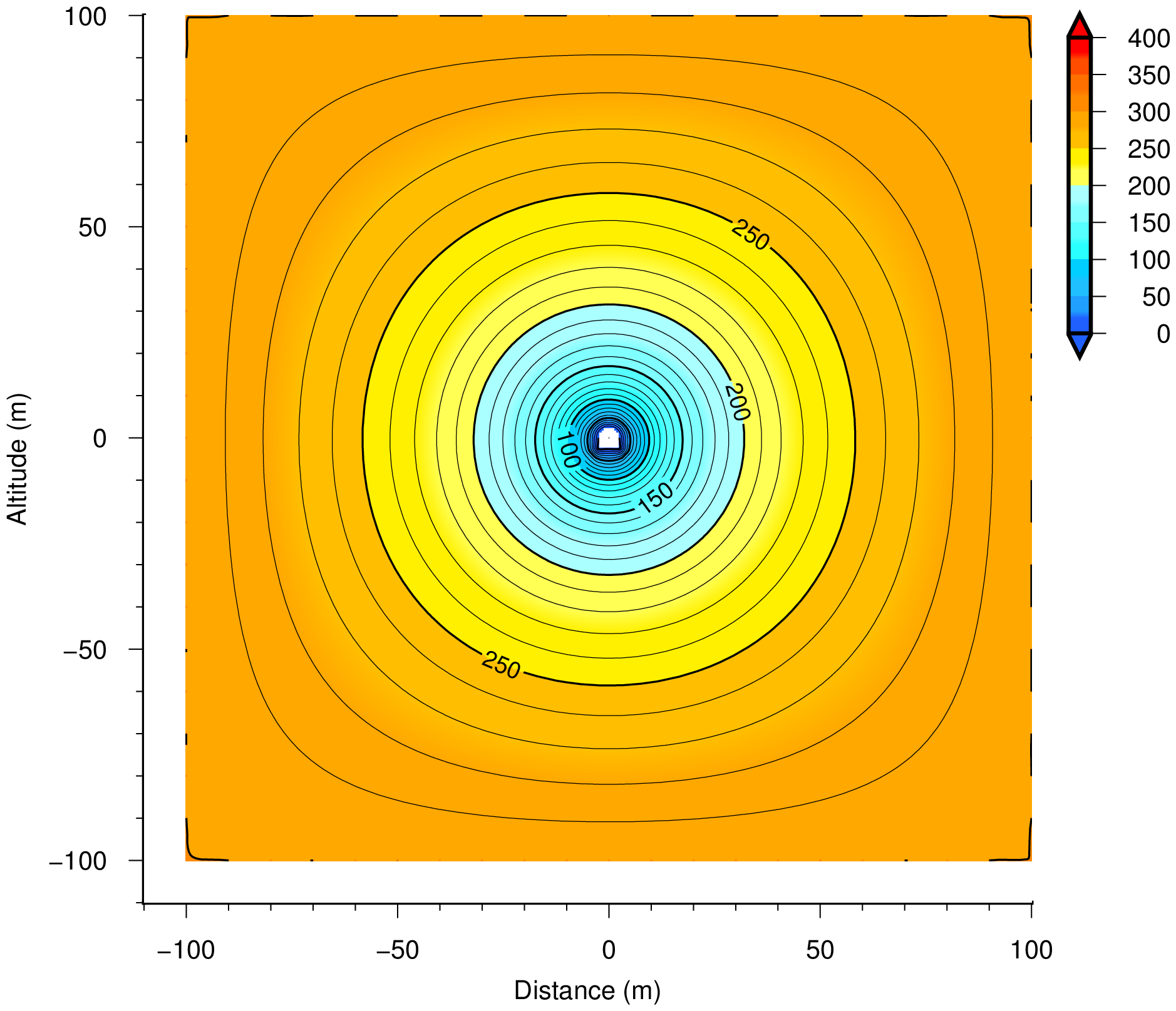
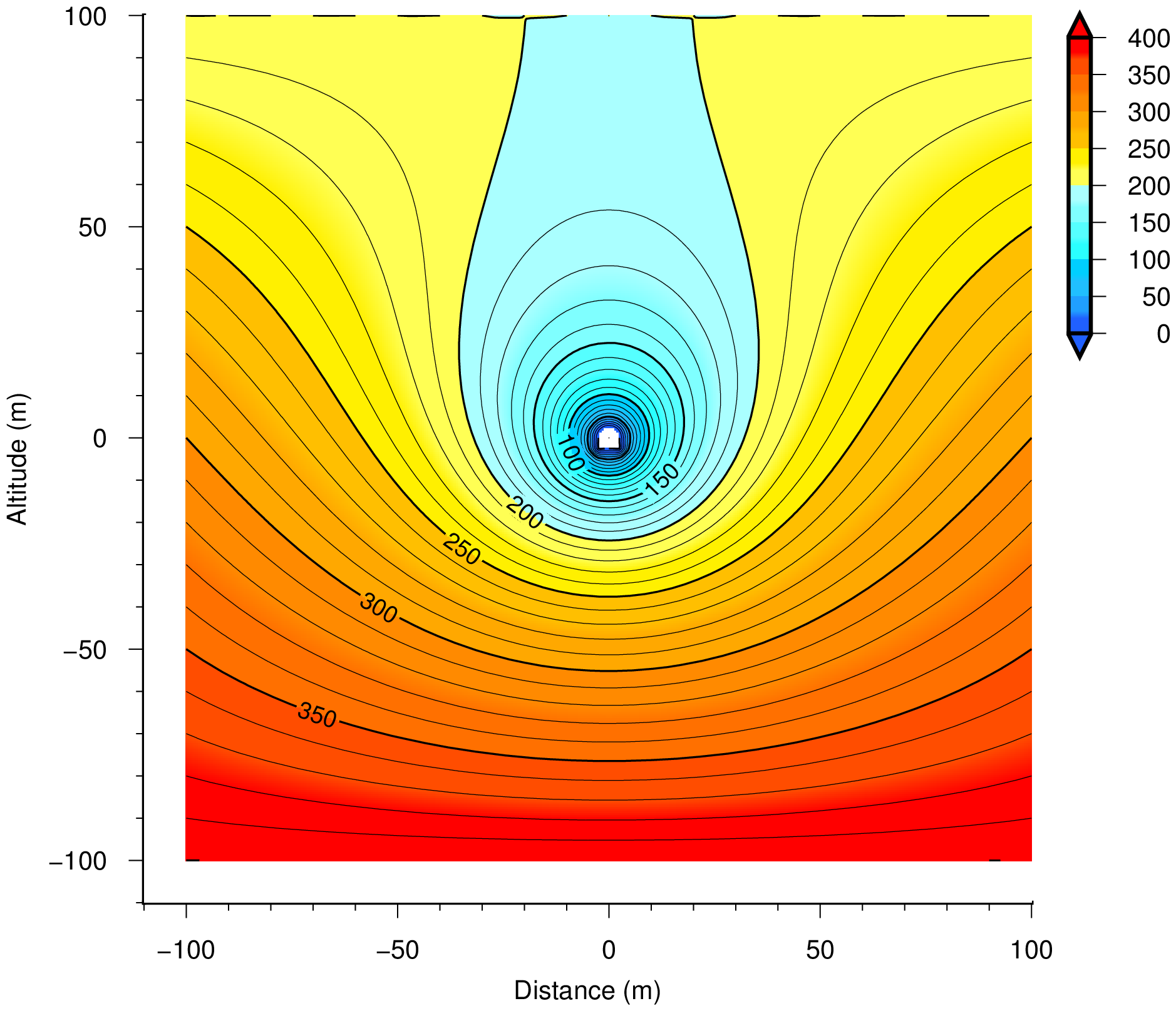
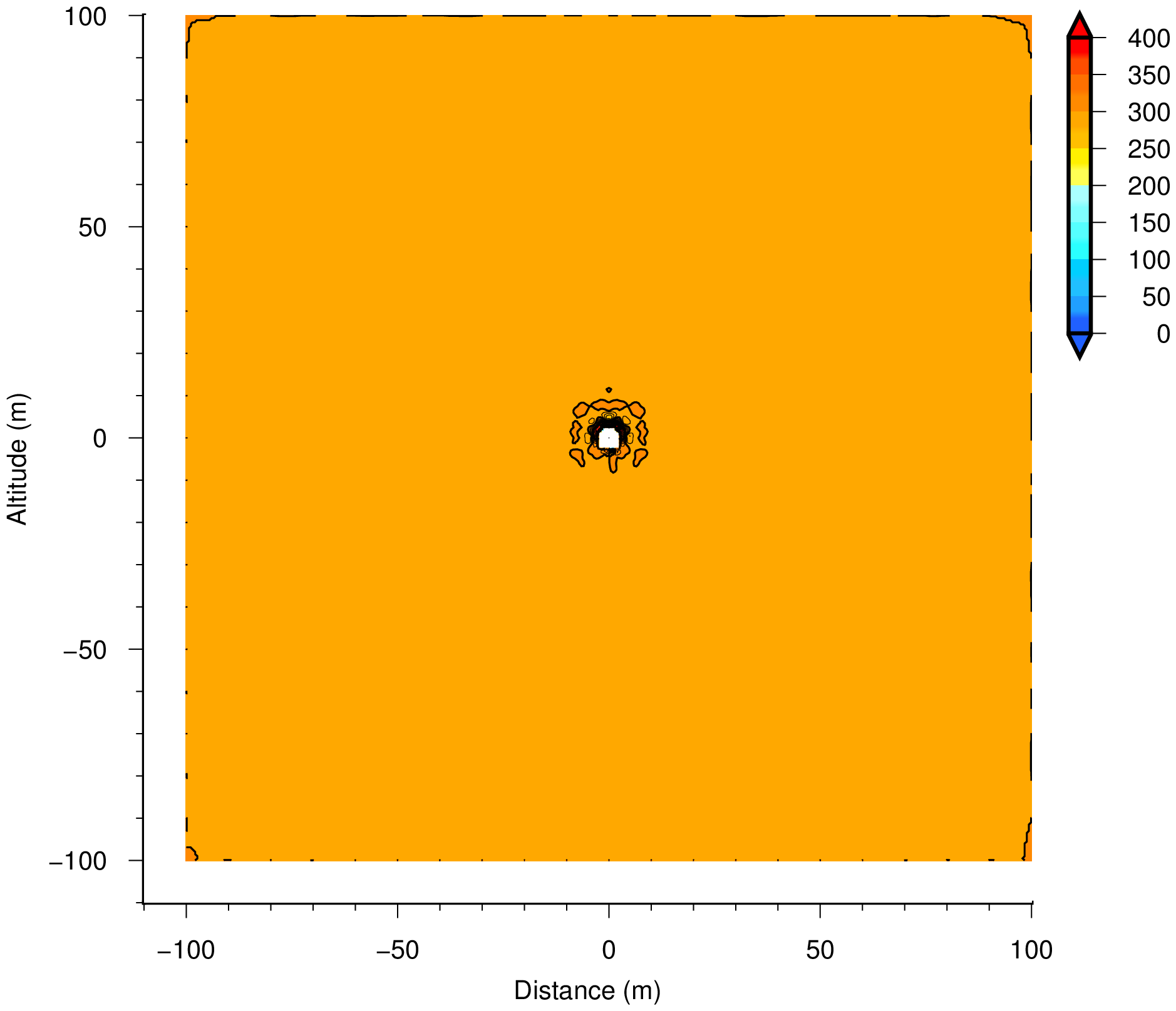
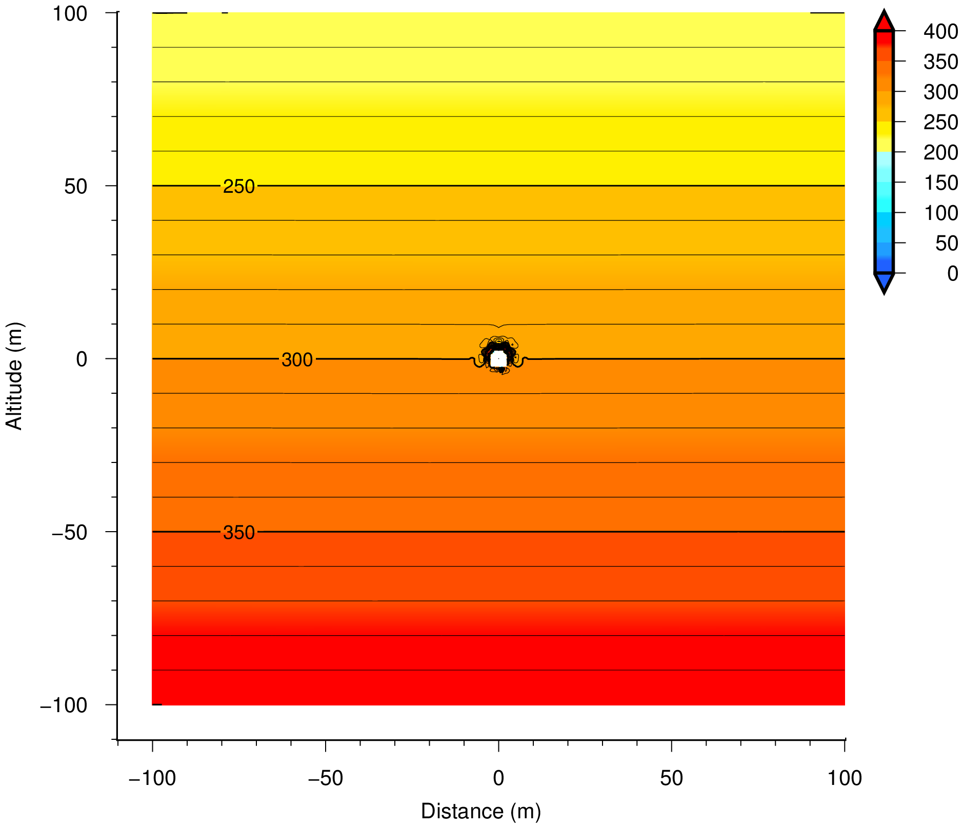
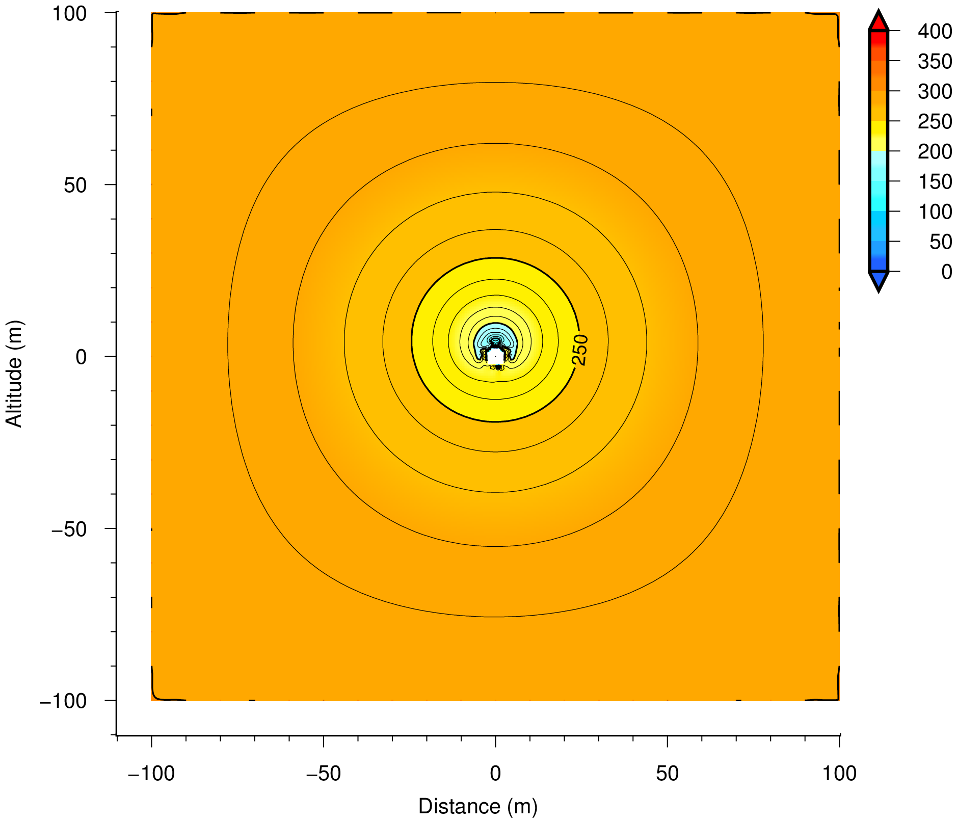
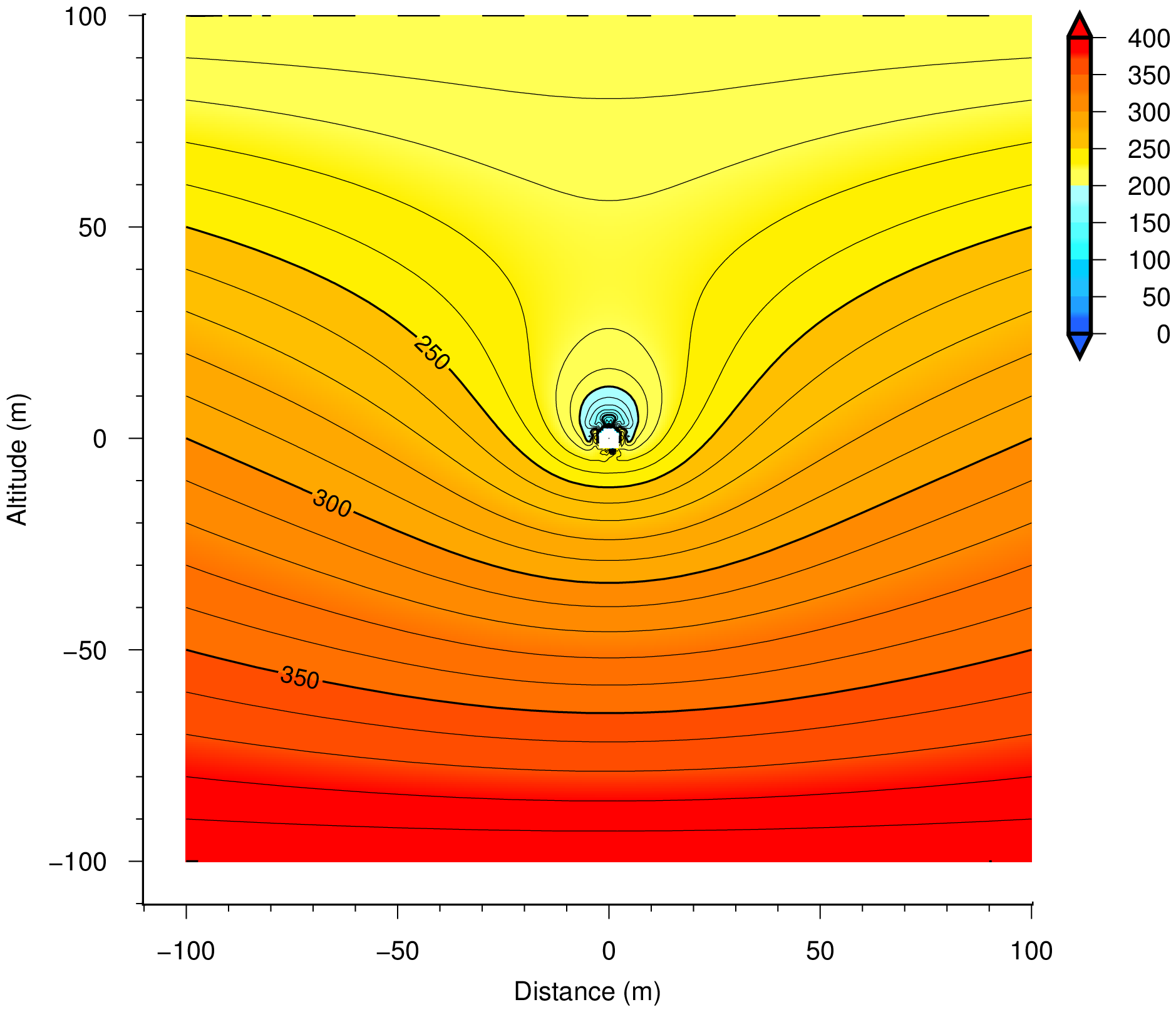
Pressure head analysis around the tunnel
- This section shows the example of analysis for tunnel under ground water.
- Domain for analysis is a square area with 200m-side.
- Tunnel is D-shape tunnel with 5m-width and 5m-height.
- Permeability of the ground rock is 1×10⁻⁷m/s and overburden of tunnel is 300m.
- Therefore, total head of 300m is acted at perimeters of analysis domain.
Cases for analysis are shown below.
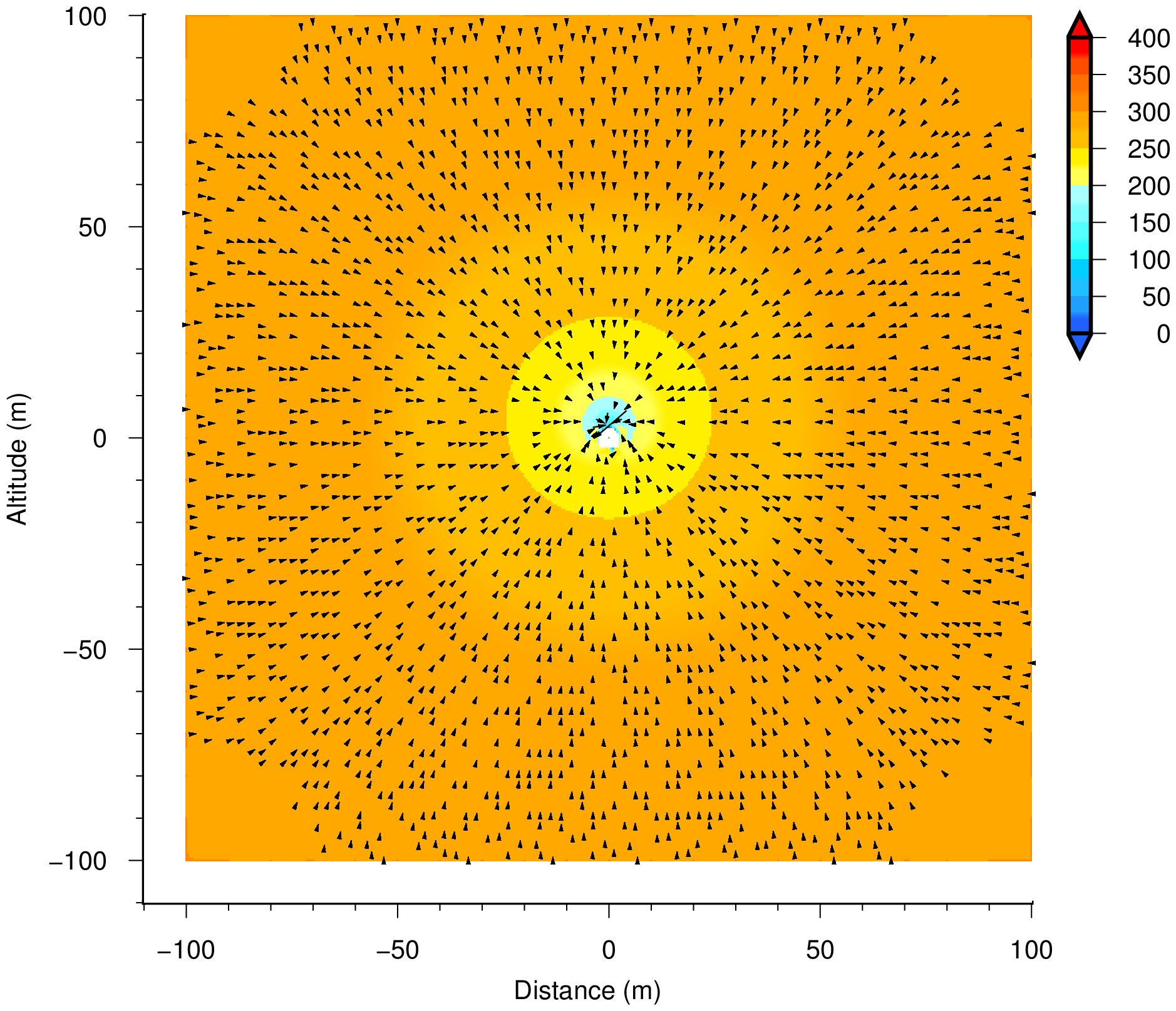
| Case-0 No-lined tunnel. | (no-lined) Wall of tunnel is ground rock. Pressure head at tunnel wall is zero. |
|---|---|
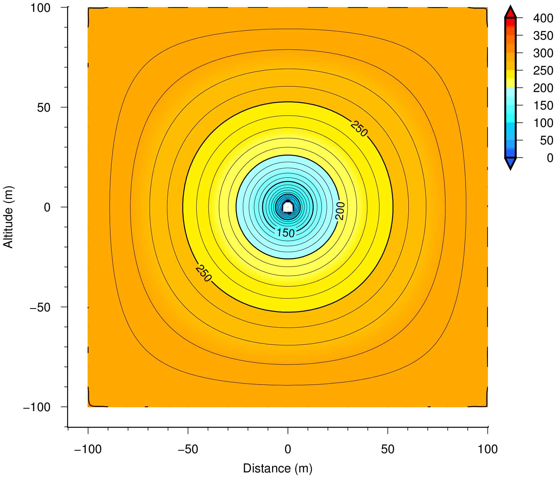
| Case-1 Tunnel with 20cm thickness concrete lining. |
(lined) Permeability of lining concrete is 1×10$^{−12}$m/s. (no-drainage) Pressure head at inner surface of concrete lining is zero. |
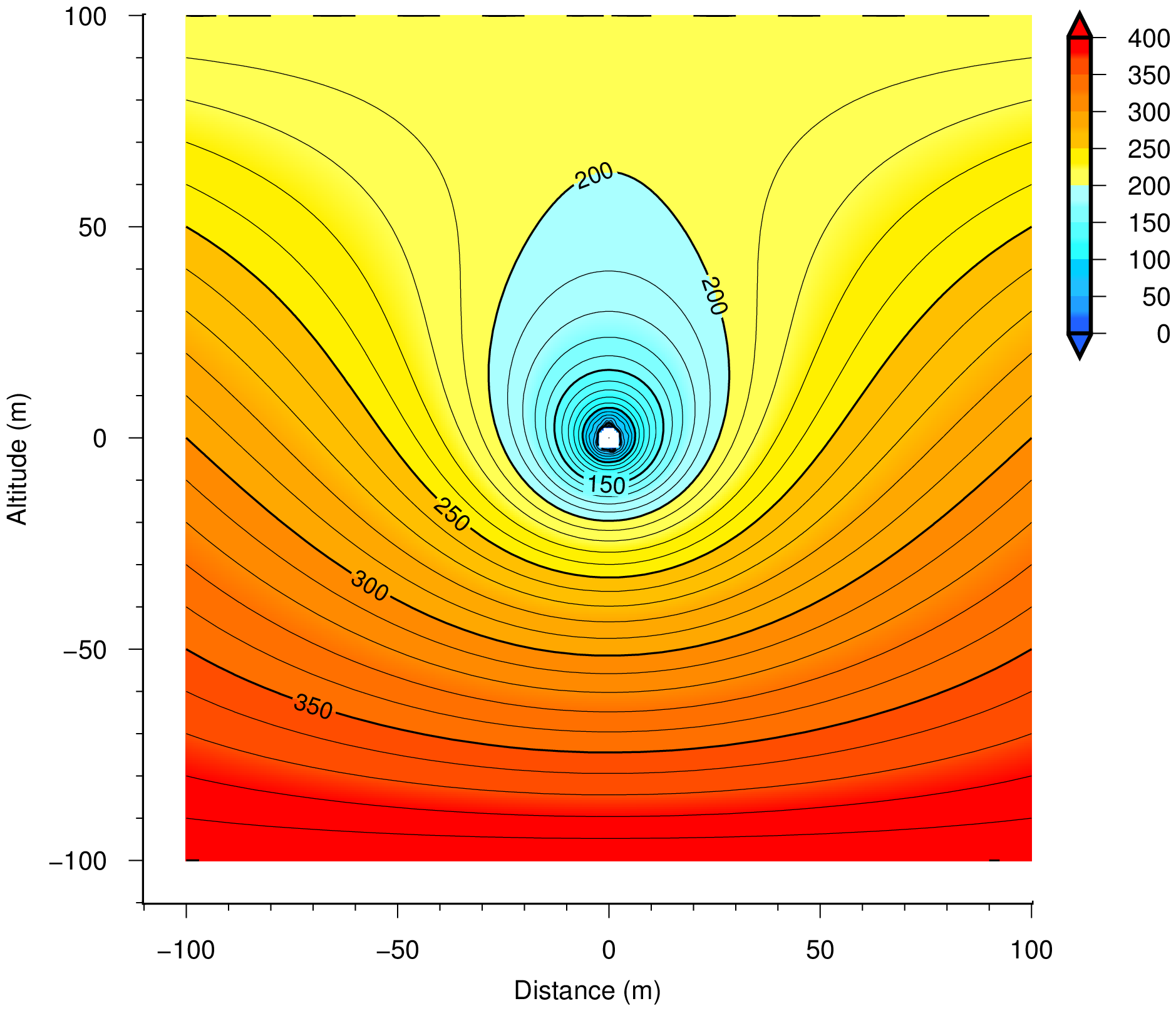
| Case-2 Tunnel with 20cm thickness concrete lining. |
(lined) Permeability of lining concrete is 1×10$^{−12}$m/s. (one drain hole) One drain hole is installed at the top of tunnel concrete lining. Pressure head at drain hole and inner surface of concrete lining is zero. |
| Case-3 Tunnel with 20cm thickness concrete lining. |
(lined) Permeability of lining concrete is 1×10$^{−8}$m/s. (one drain hole) One drain hole is installed at the top of tunnel lining concrete. Pressure head at drain hole and inner surface of concrete lining is zero. |
| Case-4 Tunnel with 20cm thickness concrete lining. |
(lined) Permeability of lining concrete is 1×10$^{−7}$m/s. (one drain hole) One drain hole is installed at the top of tunnel concrete lining. Pressure head at drain hole and inner surface of concrete lining is zero. |
 |
| Mesh |
|---|
 |
 |
 |
| Case-0 | ||
|---|---|---|
 |
 |
 |
| Case-1 | ||
 |
 |
 |
| Case-2 | ||
 |
 |
 |
| Case-3 | 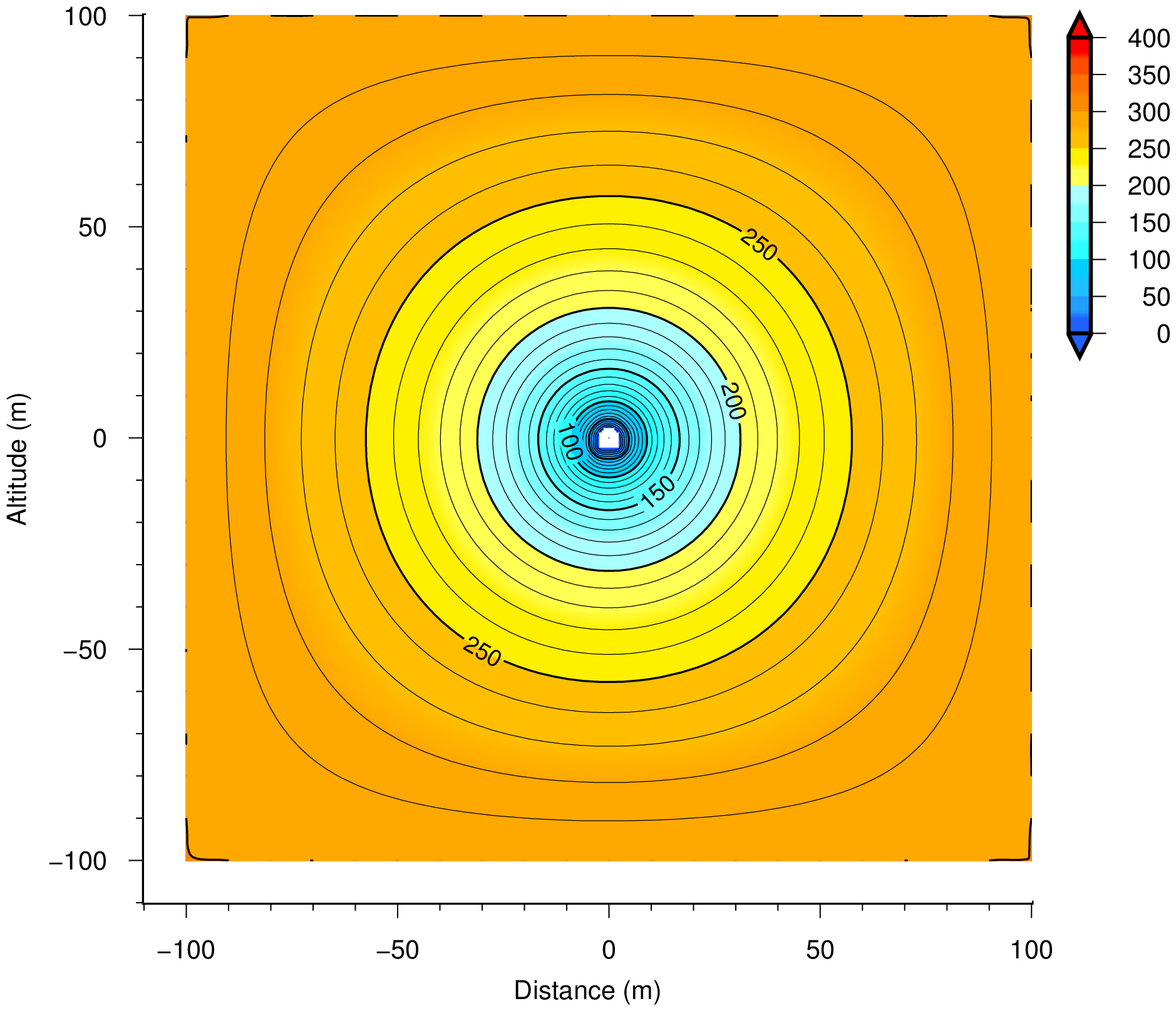 |
 |
 |
| Case-4 | ||
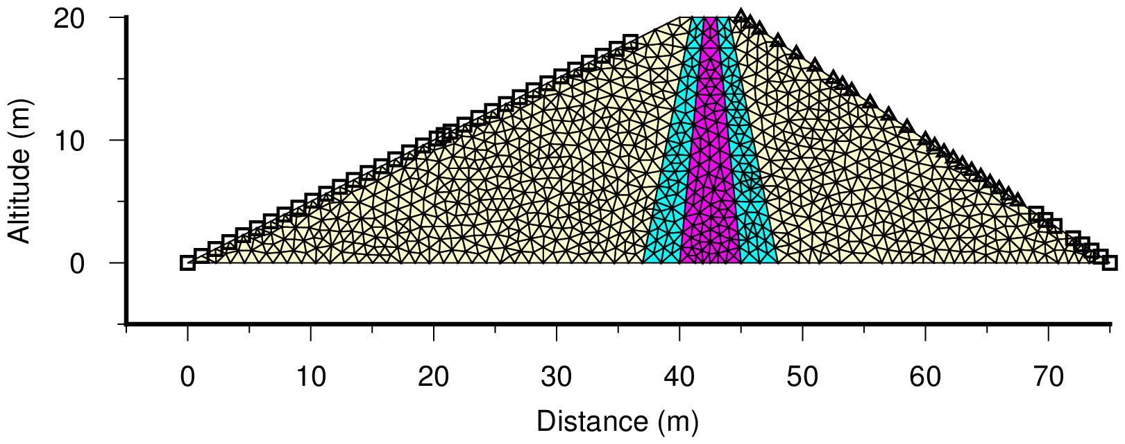
Zoned embankment dam
In this section, examples of analysis for zoned embankment dam are shown. In addition, it is a wellknown fact for zoned embank dam that the free water surface serves as an action which has a permeating point on the core back and does not become such form shown in this analysis.
<>pThe Conditions of analysis are shown in below table.| Height (m) | Top width (m) | Upstream slope | Downstream slope | Upstream Water Depth (m) | Downstream Water Depth (m) |
|---|---|---|---|---|---|
| 20.0 | 5.0 | 1:2.0 | 1:1.5 | 18.0 | 4.0 |
| Material properties | |||
|---|---|---|---|
| Zone | Permeability k (m/s) | $\alpha$ (m$^{-1}$) | m |
| Upstream shell | 1×10$^{0}$ | 0.1 | 0.7 |
| Upstream filter | 1×10$^{-4}$ | 0.1 | 0.7 |
| center core | 1×10$^{-5}$ | 0.1 | 0.7 |
| Downstream filter | 1×10$^{-4}$ | 0.1 | 0.7 |
| Downstream shell | 1×10$^{0}$ | 0.1 | 0.7 |
 |
 |
| Mesh diagram | |
|---|---|
 |
 |
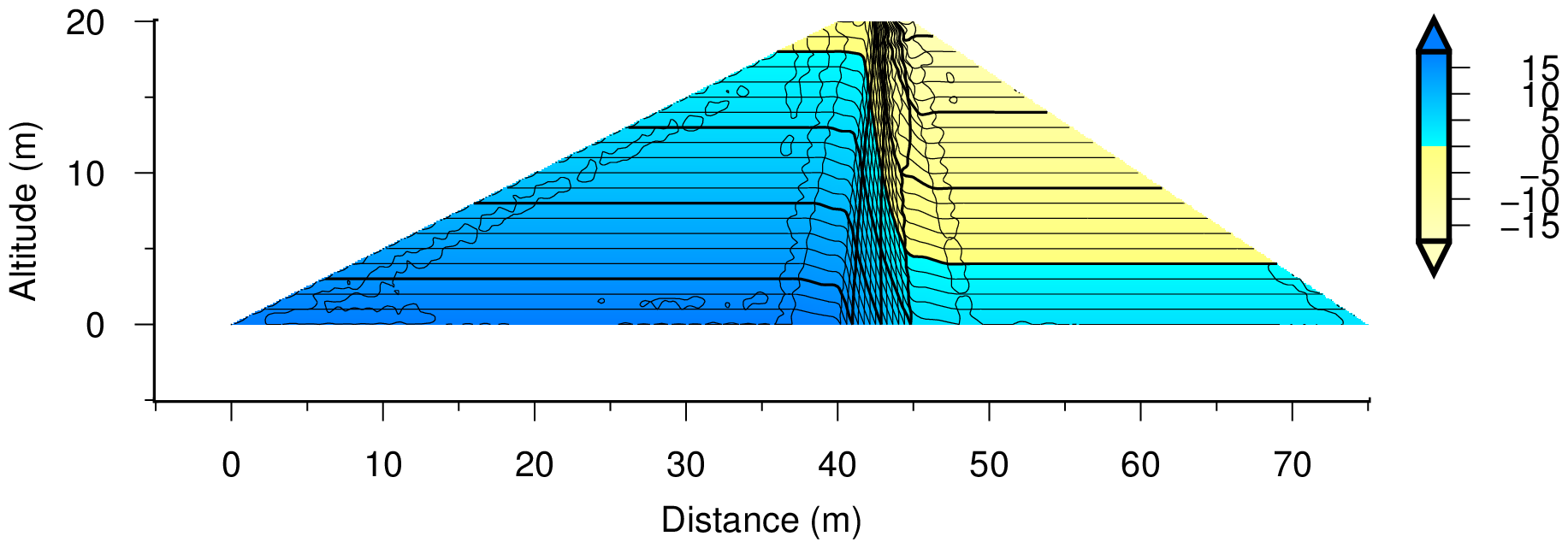
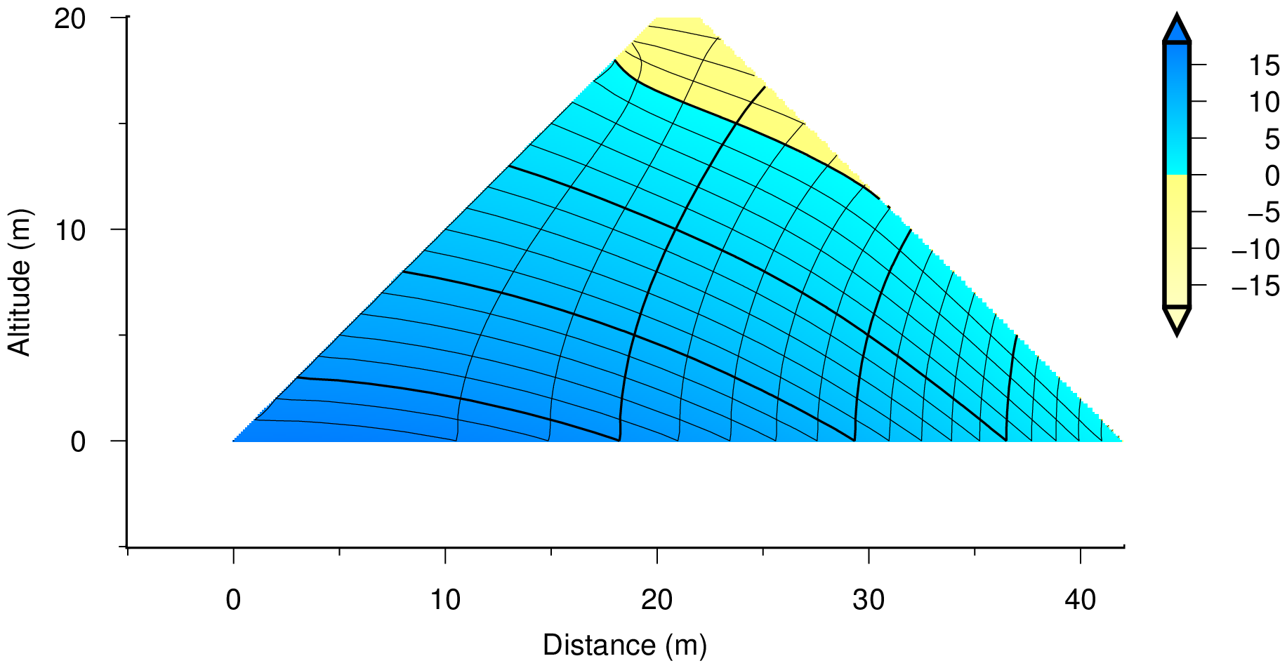
| Pressure Head Distribution | |
 |
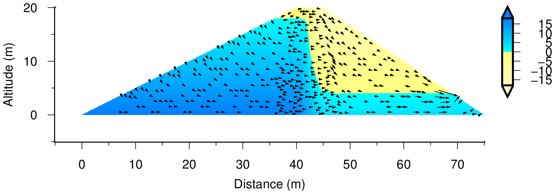 |
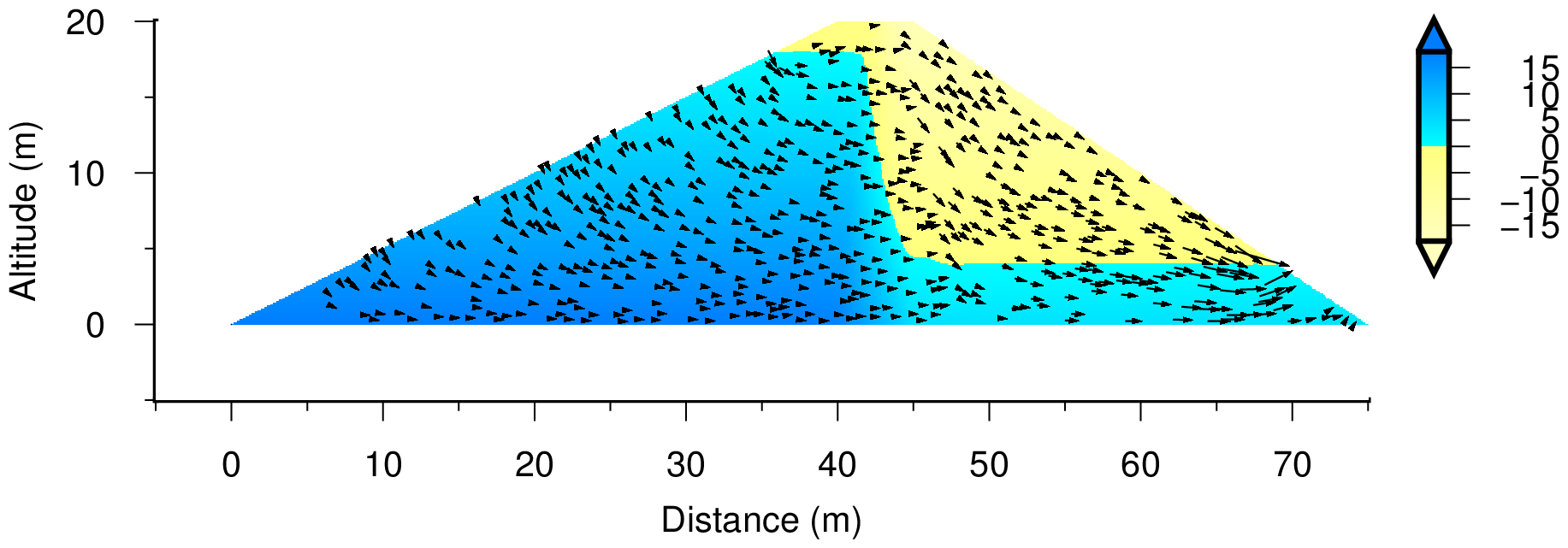
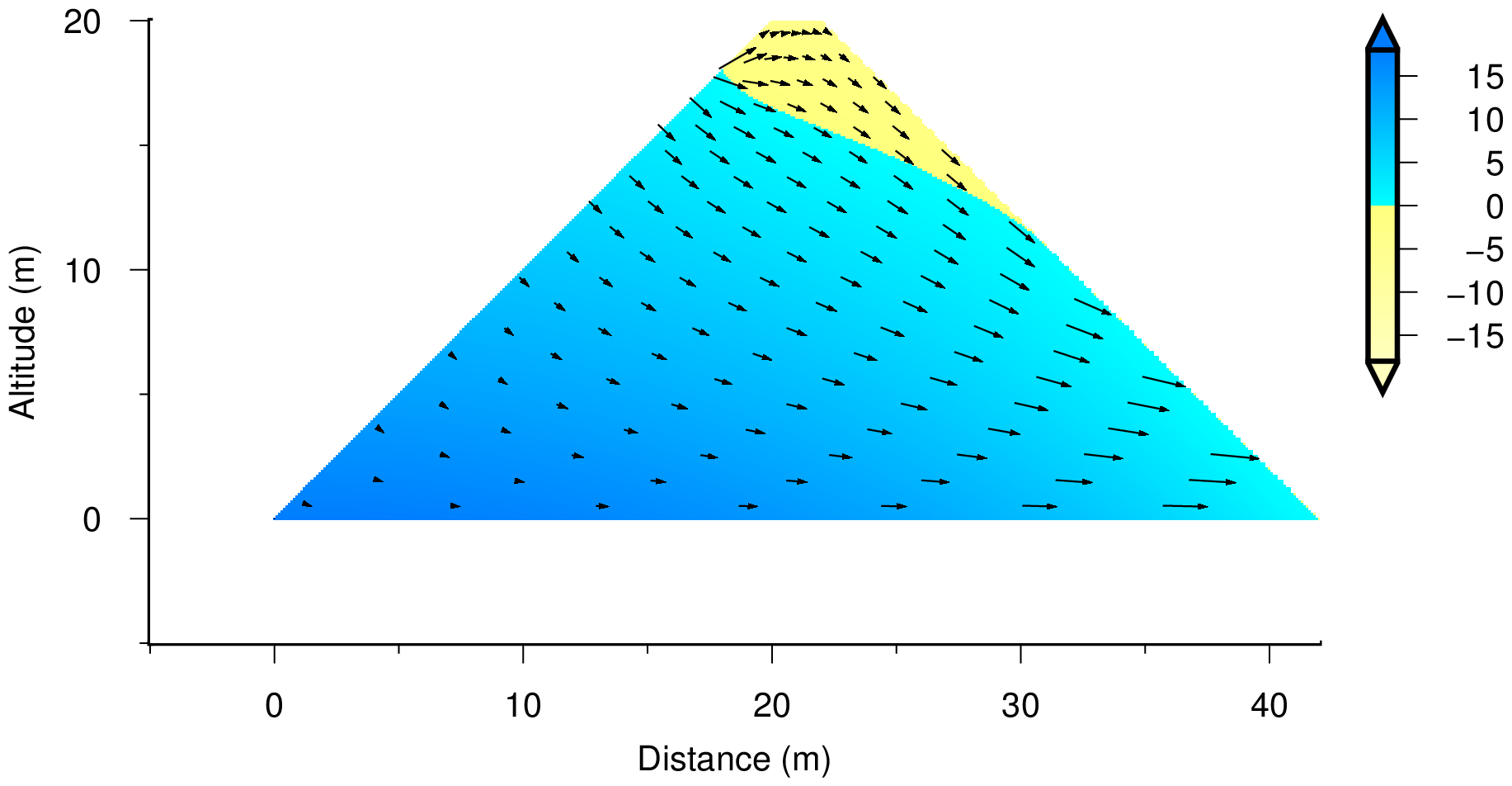
| Flow Velocity Vector | |
 |
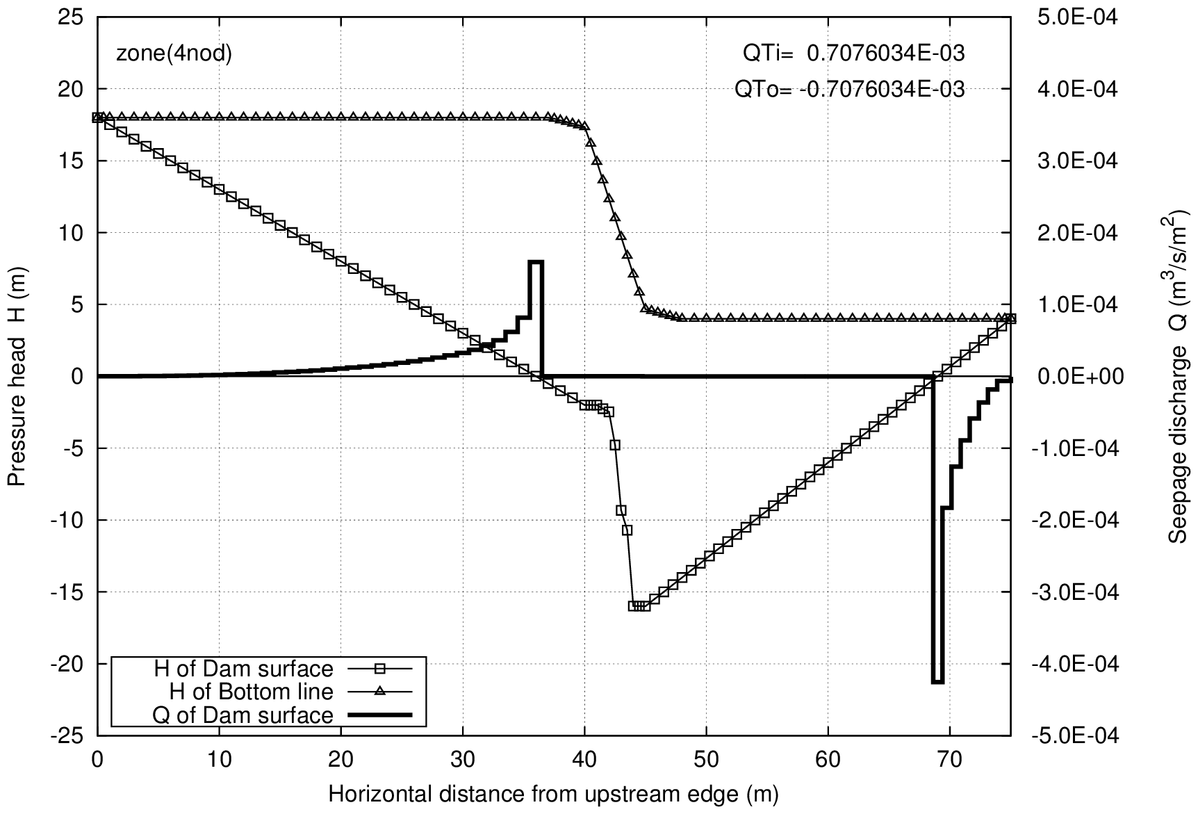 |
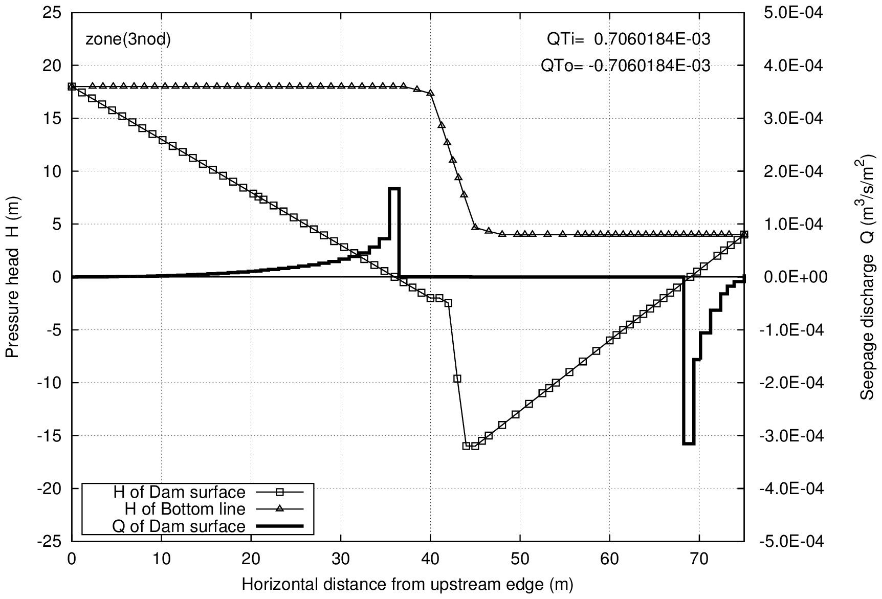
| Pressure Head and Discharge | |
Homogeneous embankment dam
The seepage flow discharge by seepage flow FEM was compared with it by Casagrande's method.
Casagrande's method
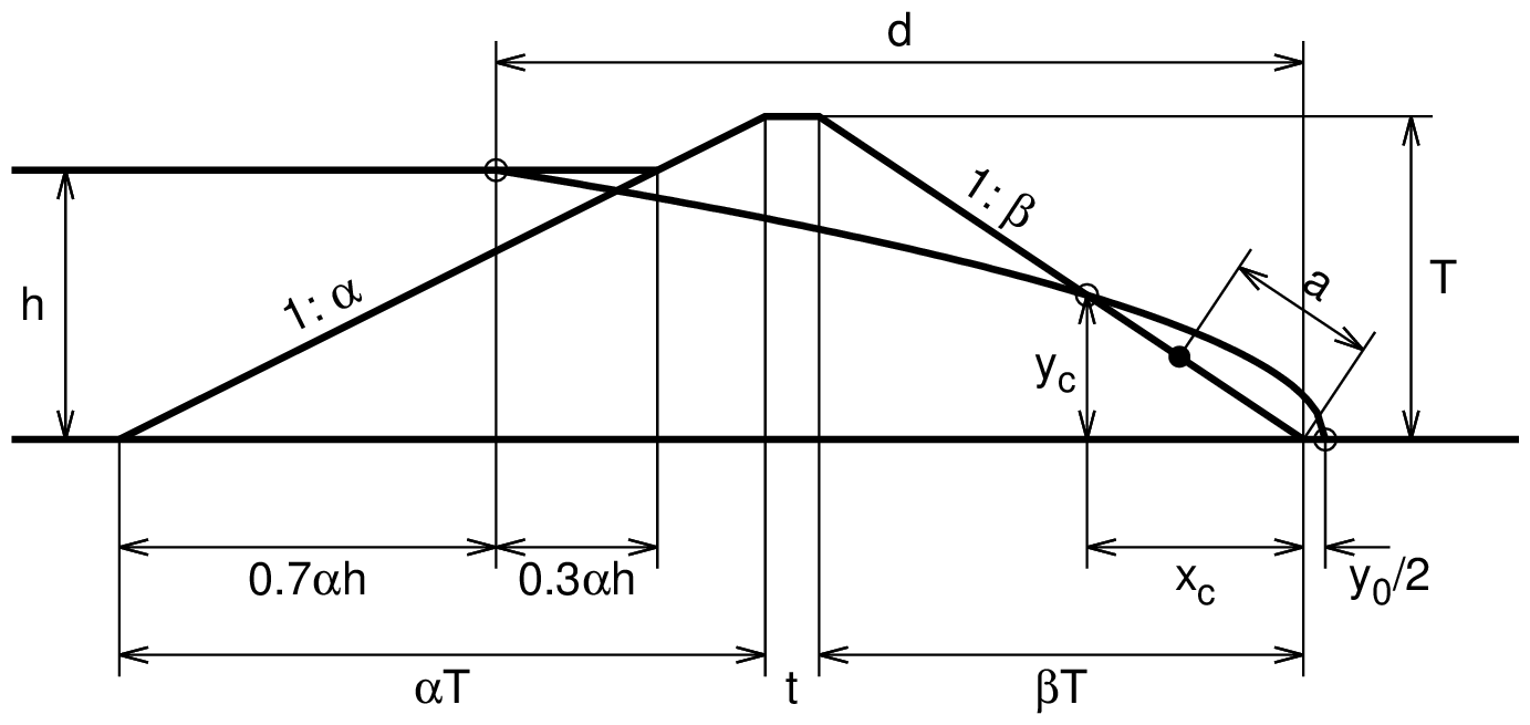 |
| Casagrande's model |
|---|
| $T$ | : Dam height |
| $t$ | : Width of dam top |
| $\alpha$ | : Gradient of upstream slope (1 : $\alpha$) |
| $\beta$ | : Gradient of downstream slope (1 : $\beta$) |
| $h$ | : Water depth of upstream |
| $k$ | : Permeability coefficient of dam body |
First approximation
\begin{align*} &d=T (\alpha+\beta)+t-0.7\cdot\alpha\cdot h \\ &a=\sqrt{d^2+h^2}-\sqrt{d^2-h^2\cdot\beta^2} \\ &q=k\cdot\frac{a}{1+\beta^2} \end{align*}Second approximation
\begin{align*} &d=T (\alpha+\beta)+t-0.7\cdot\alpha\cdot h \\ &y_0=\sqrt{d^2+h^2}-d \\ &x_c=\frac{\beta^2 h^2+\sqrt{\beta^2 h^2\{\beta^2 h^2+2(d+y_0/2)y_0\}}}{2(d+y_0/2)} \\ &y_c=\frac{x_c}{\beta} \\ &S=\sqrt{(d-x_c)^2+(h-y_c)^2}+\sqrt{x_c{}^2+y_c{}^2} \\ &a=S-\sqrt{S^2-h^2(1+\beta^2)} \\ &q=k\cdot\frac{a}{1+\beta^2} \end{align*}Since first approximation gives the result of safety side based on trial calculation, first approximation was used on the calculations in this document.
Result of seepage flow FEM
Conditions for analysis
Conditions for analysis and outline of results are shown below.
| Dam shape | Water level | Material properties | |||||
|---|---|---|---|---|---|---|---|
| Height (m) | Top width (m) | Slope | Bottom width (m) | U / D (m) | Permeability $k$ (m/s) | $\alpha$ (m$^{-1}$) | $m$ |
| 20.0 | 2.0 | 1:0.1 | 6.0 | 18.0 / 0.0 | 1$\times$10$^{-5}$ | 0.1 | 0.7 |
| 20.0 | 2.0 | 1:0.5 | 22.0 | 18.0 / 0.0 | 1$\times$10$^{-5}$ | 0.1 | 0.7 |
| 20.0 | 2.0 | 1:1.0 | 42.0 | 18.0 / 0.0 | 1$\times$10$^{-5}$ | 0.1 | 0.7 |
| 20.0 | 2.0 | 1:1.5 | 62.0 | 18.0 / 0.0 | 1$\times$10$^{-5}$ | 0.1 | 0.7 |
| 20.0 | 2.0 | 1:2.0 | 82.0 | 18.0 / 0.0 | 1$\times$10$^{-5}$ | 0.1 | 0.7 |
| 20.0 | 2.0 | 1:2.5 | 102.0 | 18.0 / 0.0 | 1$\times$10$^{-5}$ | 0.1 | 0.7 |
| 20.0 | 2.0 | 1:3.0 | 122.0 | 18.0 / 0.0 | 1$\times$10$^{-5}$ | 0.1 | 0.7 |
 |
 |
 |
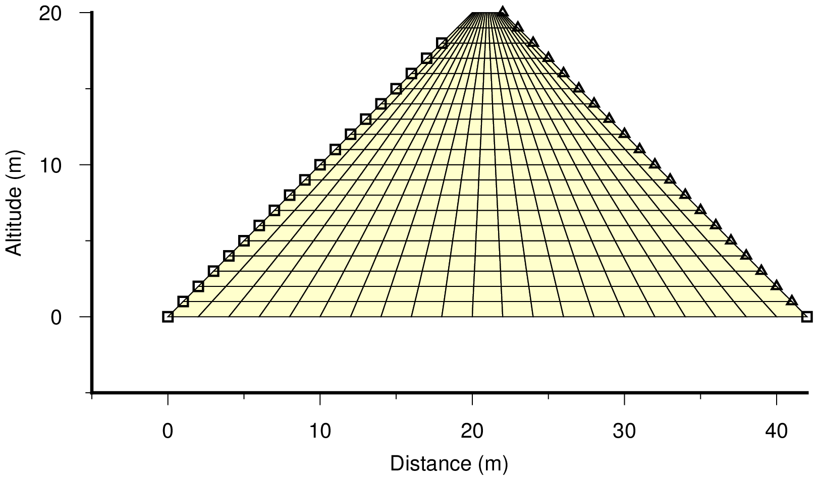
| Sample of Model of Homogeneous embankment dam | ||
|---|---|---|
Result of FEA
| 3 node element | ||||||
|---|---|---|---|---|---|---|
| Slope | Angle ($^\circ$) | Bottom width (m) | Seepage point from USE (m) | Seepage point from DSE (m) | Distance $a$ (m) | Discharge (m$^3$/s/m) |
| 1:0.1 | 84.3 | 6.0 | 4.3 | 1.7 | 17.1 | 0.3542$\times$10$^{-3}$ |
| 1:0.5 | 63.4 | 22.0 | 15.0 | 7.0 | 15.6 | 0.1178$\times$10$^{-3}$ |
| 1:1.0 | 45.0 | 42.0 | 31.0 | 11.0 | 15.6 | 0.7112$\times$10$^{-4}$ |
| 1:1.5 | 33.7 | 62.0 | 46.0 | 16.0 | 19.2 | 0.5327$\times$10$^{-4}$ |
| 1:2.0 | 26.6 | 82.0 | 60.5 | 21.5 | 24.0 | 0.4256$\times$10$^{-4}$ |
| 1:2.5 | 21.8 | 102.0 | 75.0 | 27.0 | 29.1 | 0.3550$\times$10$^{-4}$ |
| 1:3.0 | 18.4 | 122.0 | 90.0 | 32.0 | 33.7 | 0.3093$\times$10$^{-4}$ |
| 4 node element | ||||||
| Slope | Angle ($^\circ$) | Bottom width (m) | Seepage point from USE (m) | Seepage point from DSE (m) | Distance $a$ (m) | Discharge (m$^3$/s/m) |
| 1:0.1 | 84.3 | 6.0 | 4.3 | 1.7 | 17.1 | 0.3533$\times$10$^{-3}$ |
| 1:0.5 | 63.4 | 22.0 | 15.2 | 6.8 | 15.2 | 0.1169$\times$10$^{-3}$ |
| 1:1.0 | 45.0 | 42.0 | 30.5 | 11.5 | 16.3 | 0.6957$\times$10$^{-4}$ |
| 1:1.5 | 33.7 | 62.0 | 46.0 | 16.0 | 19.2 | 0.5084$\times$10$^{-4}$ |
| 1:2.0 | 26.6 | 82.0 | 61.0 | 21.0 | 23.5 | 0.4030$\times$10$^{-4}$ |
| 1:2.5 | 21.8 | 102.0 | 76.0 | 26.0 | 28.0 | 0.3345$\times$10$^{-4}$ |
| 1:3.0 | 18.4 | 122.0 | 93.0 | 29.0 | 30.6 | 0.2864$\times$10$^{-4}$ |
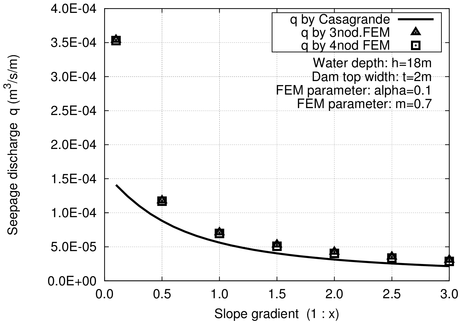
Result of comparison
Following matters are cleared from figures.
- The seepage flow discharge $Q$ by FEM is greater than it by Casagrande's method for each case.
- If the slope becomes steep, the difference of discharge between FEM and Casagrande's method becomes large.
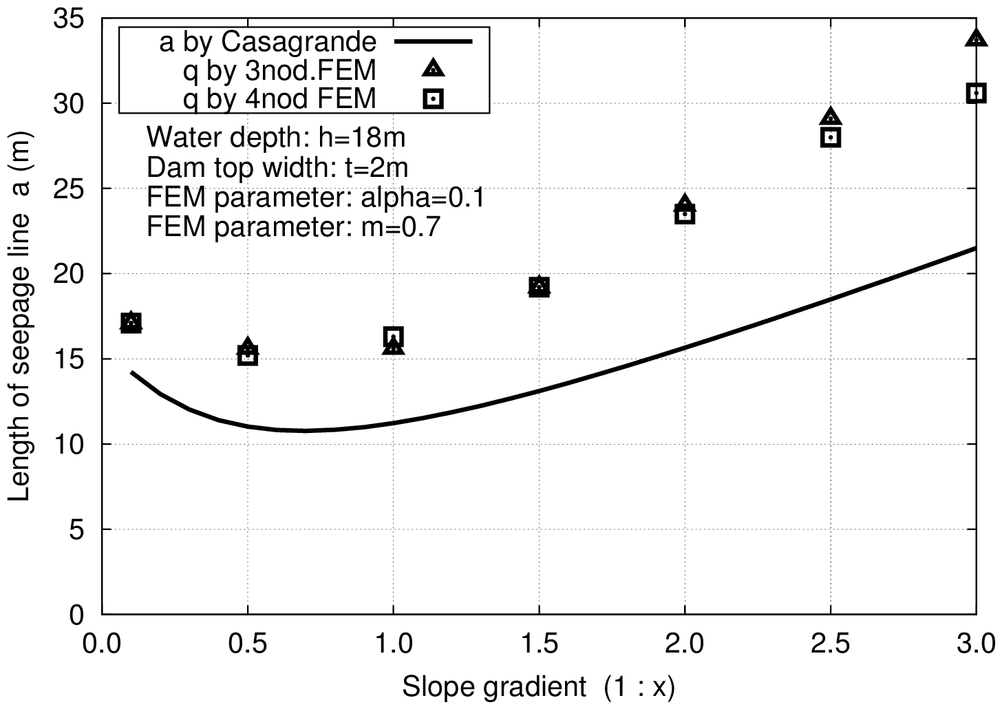
- The distance $a$ from downstream edge of dam to seepage point by FEM is greater than it of Casagrande's method for each.
- If the slope becomes gentle, the difference of distance 'a' between FEM and Casagrande's method becomes large.
 |
 |
| Discharge $Q$-Slope relationship on Homogeneous embankment dam |
Distance $a$-Slope relationship on Homogeneous embankment dam |
|---|
Programs and sample data
Fortran programs
| Filename | Description |
|---|---|
| f90_fem_seep.f90 | Seepage Analysis |
| f90_num_seep.f90 | Node number optimization |
| f90_gmt_seep.f90 | GMT drawing |
| f90_pq.f90 | gnuplot drawing of Dam Pressure Head and Node Discharge |
Shell scripts
| Filename | Description |
|---|---|
| a_fem_dam.txt | Shell script for execution of Dam seepage analysis |
| a_draw_dam.txt | Shell script for drawing of Dam seepage analysis (GMT) |
| a_dam_pq.txt | Shell script for drawing of Dam pressure head and node discharge (gnuplot) |
| a_fem_tunnel.txt | Shell script for execution of Tunnel seepage analysis |
| a_draw_tunnel.txt | Shell script for drawing of Tunnel seepage analysis |
Input data sample for dam analysis
| Filename | Description |
|---|---|
| inp_fem_zone3.csv | Zoned dam model with 3 nodes elements (original) |
| inp_fem_zone4.csv | Zoned dam model with 4 nodes elements (original) |
| inp_fem_zone3m.csv | Zoned dam model with 3 nodes elements (optimized) |
| inp_fem_zone4m.csv | Zoned dam model with 4 nodes elements (optimized) |
| inp_test0_3.csv | Homogeneous dam model with 4 nodes elements |
Input data sample for tunnel analysis
| Filename | Description |
|---|---|
| inp_tunnel_00.csv | Tunnel model Case-0 (original) |
| inp_tunnel_11.csv | Tunnel model Case-1 (original) |
| inp_tunnel_22.csv | Tunnel model Case-2 (original) |
| inp_tunnel_33.csv | Tunnel model Case-3 (original) |
| inp_tunnel_44.csv | Tunnel model Case-4 (original) |
| inp_tunnel_0m.csv | Tunnel model Case-0 (optimized) |
| inp_tunnel_1m.csv | Tunnel model Case-1 (optimized) |
| inp_tunnel_2m.csv | Tunnel model Case-2 (optimized) |
| inp_tunnel_3m.csv | Tunnel model Case-3 (optimized) |
| inp_tunnel_4m.csv | Tunnel model Case-4 (optimized) |
Expression of result of seepage flow analysis (f90_gmt_seep.f90)
Outline
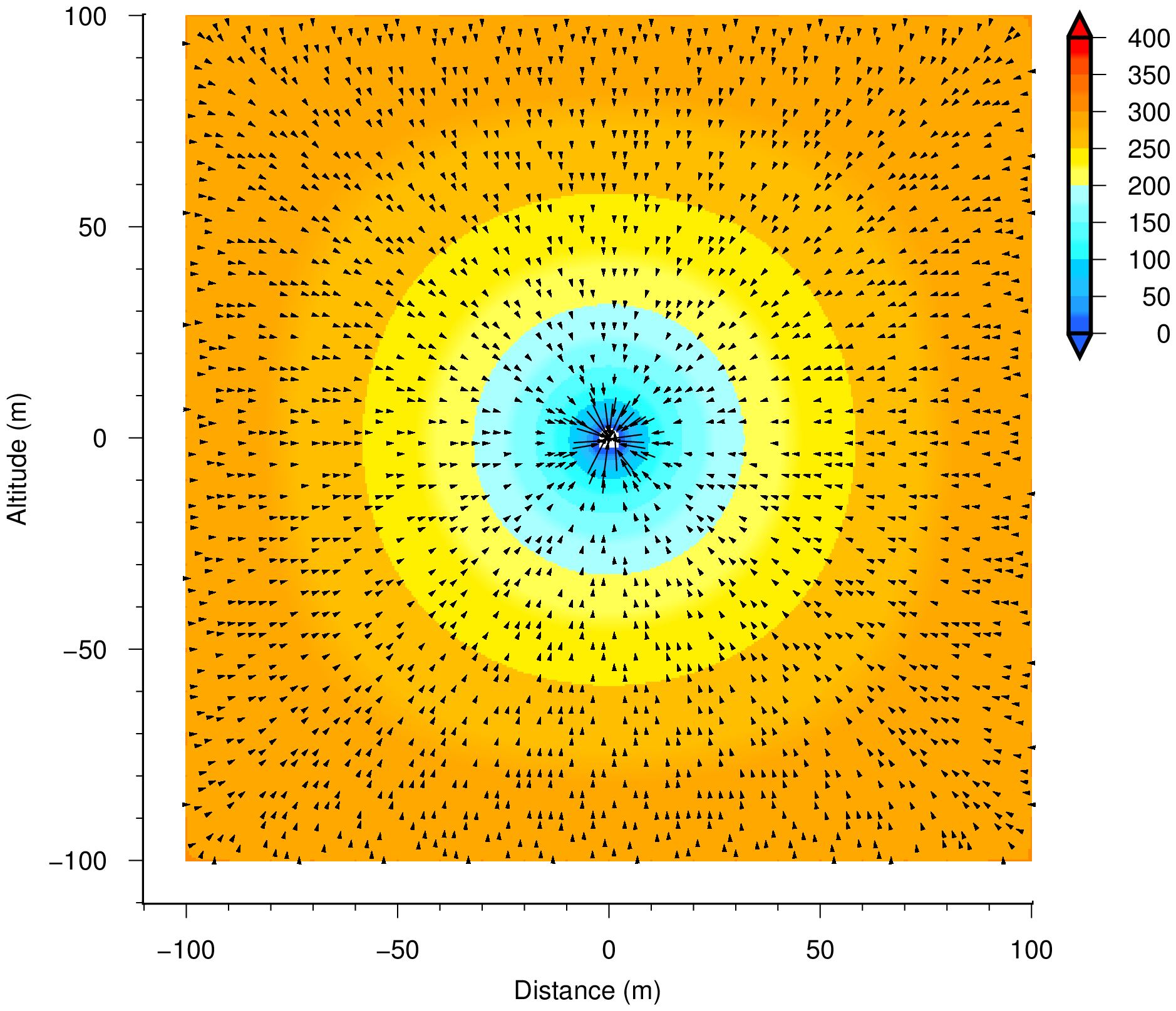
This program can show the FEM mesh, pressure head contour map, total head contour map and flow velocity vector map by using GMT.
Some explanations are shown below.
- FEM mesh is drawn by specifying the coordinates of each element and repeating painting out of each element and drawing of each element boundary line.
- The contour map is created in the following procedures.
- Creation of the mask file which defines the element existence domain by 'grdmask' command.
- Creation of the grid file for contours by 'surface' command.
- Creation of the grid file for plot by composition of the mask file and the grid file by 'grdmath' command.
- Coloring by 'grdimage' command and contour drawing by 'grdcontour' command.
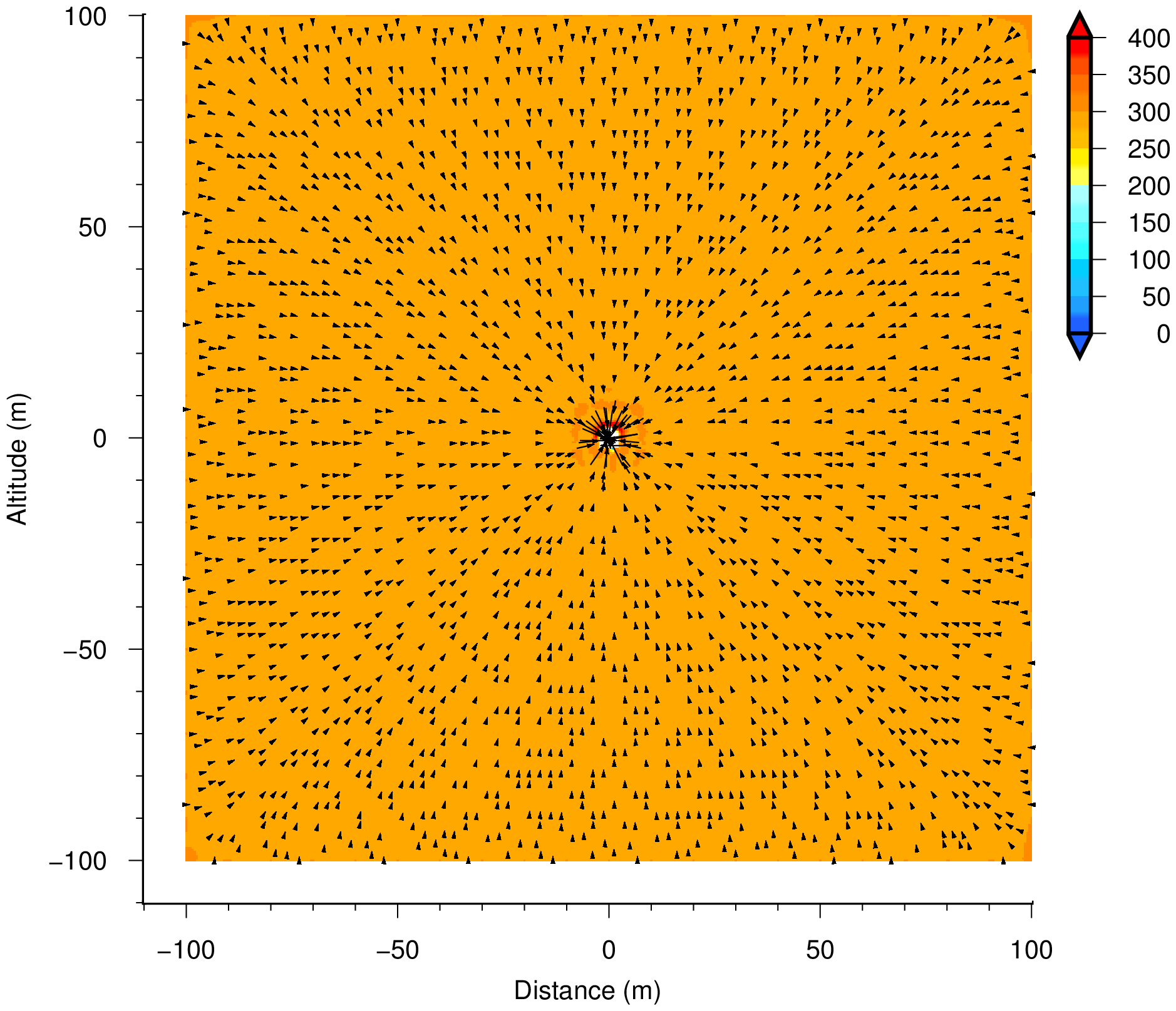
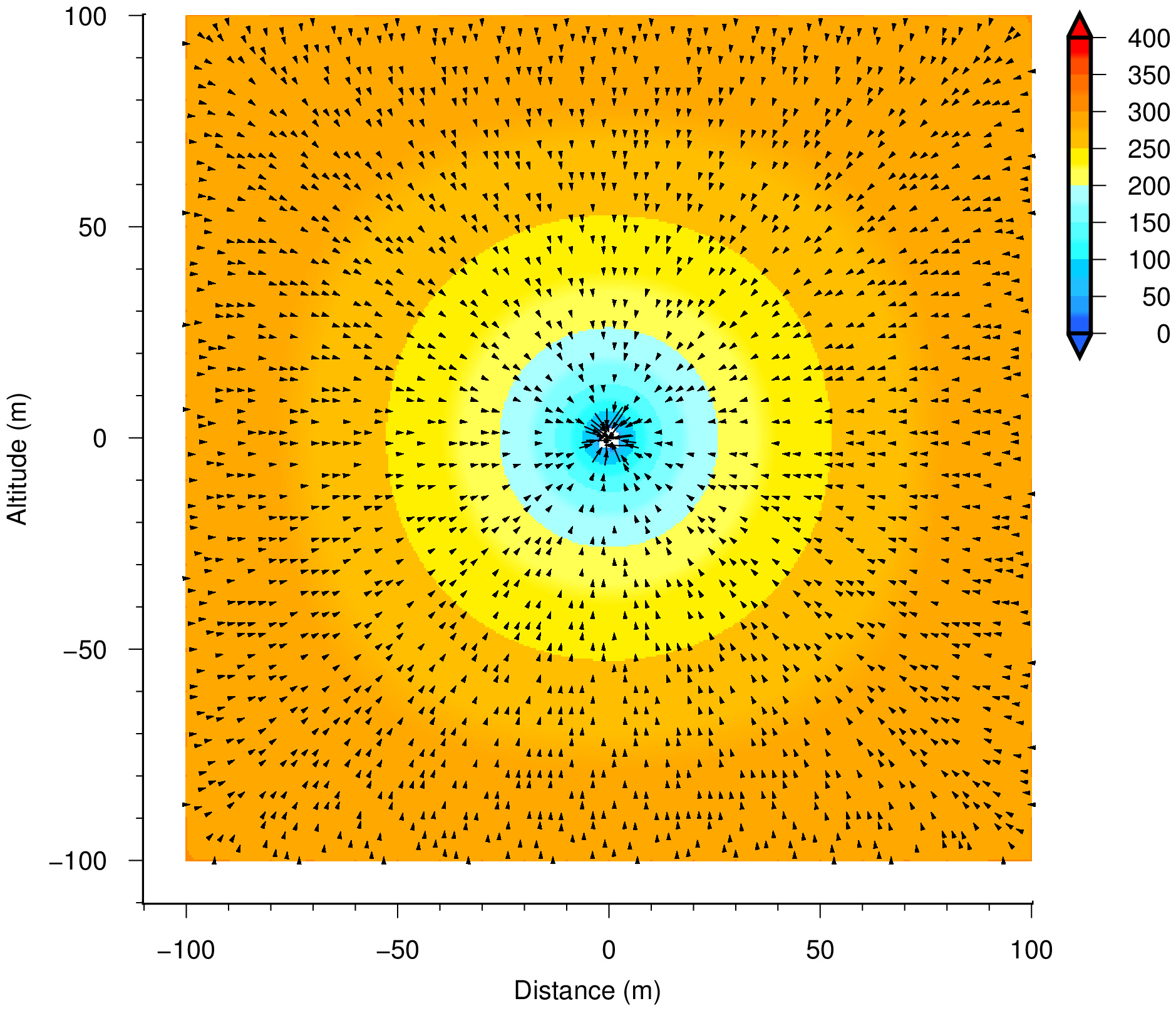
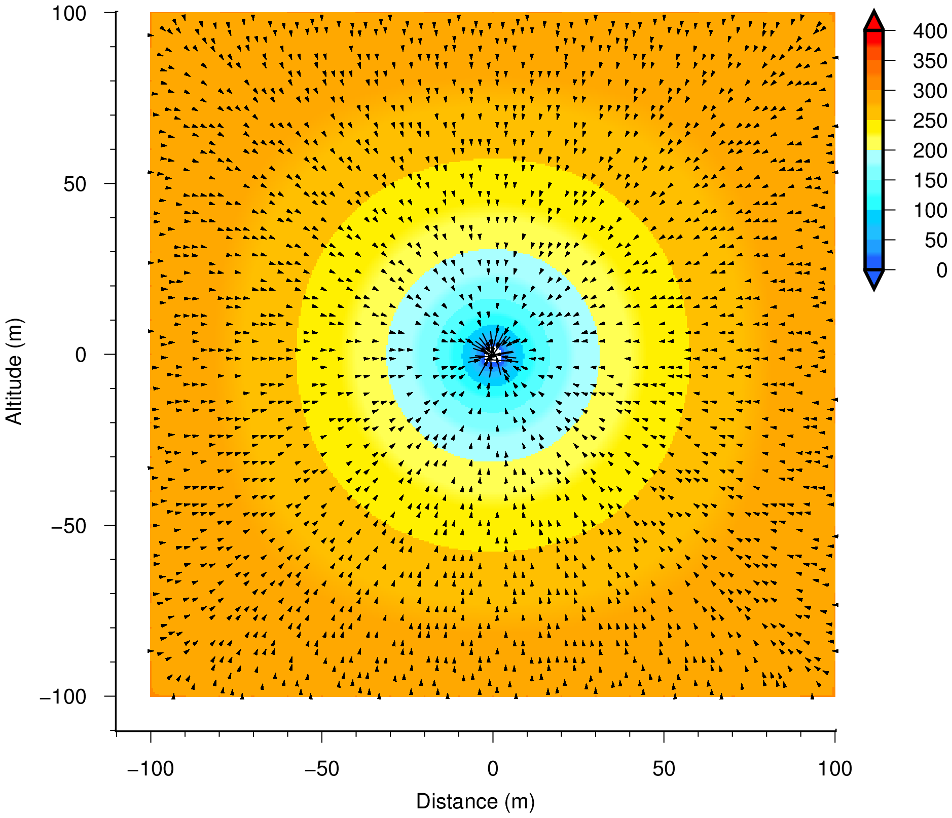
- The vector diagram is created by superimposing the arrow of the flow velocity vector on the colored map of the pressure head or total head generated by contour creation.
- In addition, since a figure will become ugly if the flow velocity vector is drawn on all elements, in this example, the flow velocity vector is drawn once per three elements.
Following files must be prepared before execution of the program.
| Filename | Description | Remarks |
|---|---|---|
| _col_mesh.txt | Input file for defining mesh color | Filename is fixed |
| _inp_base.txt | Input file for drawing information | Filename is fixed |
| 0_cpt.cpt | Input cpt file for reading by GMT | Filename is fixed |
| fnameW.csv | Output file by FEM analysis | Filename is changeable |
Output file by FEM analysis is a output by the program 'f90_fem_seep' made by webmaster.
Description of Shell script
Shell script (a_draw_dam.txt) which carries out the process is shown below. Some files which are read from Fortran program are made in this batch file.
001   gfortran -o f90_gmt_seep f90_gmt_seep.f90
002
003   cp 0_cpt_dam.cpt 0_cpt.cpt
004
005   # define of mesh colour (1:MATEL)
006   cat << EOT > _col_mesh.txt
007   255 255 204
008     0 255 255
009   255   0 255
010     0 255 255
011   255 255 204
012   EOT
013   # integer::ind,ibc,iph,ivc,isc
014   # real(4)::baselength,grdspc
015   # real(4)::bav,bfv
016   # real(4)::conint,annint
017   # character::strx*100,strz*100
018   cat << EOT > _inp_base.txt
019   0 1 1 1 1
020   12.0 0.1
021   10.0 5.0
022    1.0 5.0
023   "Distance (m)"
024   "Altitude (m)"
025   EOT
026
027   ./f90_gmt_seep out_fem_zone3m.csv
028   mv -f _fig_gmt_mesh.eps fig_gmt_3mesh_dam.eps
029   mv -f _fig_gmt_conp.eps fig_gmt_3conp_dam.eps
030   mv -f _fig_gmt_vect.eps fig_gmt_3vect_dam.eps
031
032   ./f90_gmt_seep out_fem_zone4m.csv
033   mv -f _fig_gmt_mesh.eps fig_gmt_4mesh_dam.eps
034   mv -f _fig_gmt_conp.eps fig_gmt_4conp_dam.eps
035   mv -f _fig_gmt_vect.eps fig_gmt_4vect_dam.eps
036
037   ./f90_gmt_seep out_test0_3.csv
038   mv -f _fig_gmt_mesh.eps fig_gmt_mesh_earth.eps
039   mv -f _fig_gmt_conp.eps fig_gmt_conp_earth.eps
040   mv -f _fig_gmt_vect.eps fig_gmt_vect_earth.eps
041
042   rm _*
001
To compile the program 'f90_GMTseep.f90'
003
To copy '0_cpt_dam.cpt' which has been prepared beforehand to '0_cpt.cpt.' The contents of file '0_cpt_dam.cpt' is shown below.
-18 255 255 190  0 255 255 125
  0   0 255 255 18   0 125 255
B   255 255 190
F     0 125 255
N   255 255 255  N 255 255 255
006-012
To make the file '_col_mesh.txt.' Mesh colors are defined by this file, 3 figures means 'R G B' in this file. In this example, new file is made using 'cat' hear documents in this script, and since 5 materials are used (parameter MATEL=5), 5 kinds of color is defined.
018-025
To make the file '_inp_base.txt.' This file defines the parameter for GMT.
| ind | Draw node number and element number in FEM mesh. (0: no, 1: yes) |
| ibc | Draw boundary conditions in FEM mesh. (0: no, 1: yes) |
| iph | Superimpose total head line on pressure head contour, or reverse. (0: no, 1: yes) |
| ivc | Specify the kind of contour map superimposed on velocity vector map (1: pressure head contour, 2: total head contour) |
| isc | Draw scale map for contour (0: no, 1: yes) |
| baselength | Size of drawing in unit of 'cm' |
| grdspc | Mesh interval for 'grd' file |
| bav | Value of 'a' in '-B' option for x and y-axis on GMT |
| bfv | Value of 'f' in '-B' option for x and y-axis on GMT |
| conint | Value of interval of contour in '-C' option of 'grdcontour' command |
| annint | value of interval of tickmark in '-A' option of 'grdcontour' command |
| strx | Label for x(horizontal)-axis. Double prime (") is required because of character |
| strz | Label for z(vertical)-axis. Double prime (") is required because of character |
027
To execute the program 'f90_gmt_seep.' Functions of this program are to make GMT command files, to execute them and to make eps drawings.
Input file 'out_fem_zone4m.csv' which storages the result of FEM analysis is read from command line.
Output drawings are shown below.
| Filename | Description | Remarks |
|---|---|---|
| _fig_gmt_mesh.eps | FEM mesh drawing in eps format | Output filename is fixed |
| _fig_gmt_conp.eps | Pressure head contour map in eps format | Output filename is fixed |
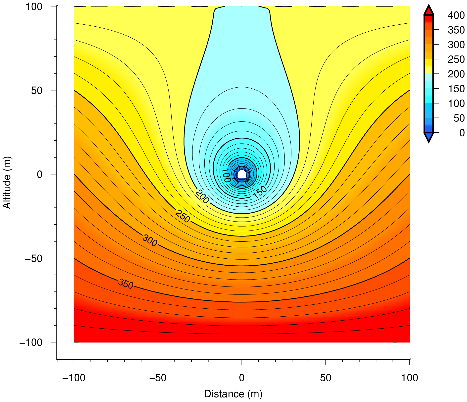
| _fig_gmt_conh.eps | Total head contour map in eps format | Output filename is fixed |
| _fig_gmt_vect.eps | Velocity vector map in eps format. | Output filename is fixed |
| Symbols for boundary conditions in FEM mesh drawing | |
|---|---|
| Symbol | Description |
| □ | Boundary of given total head |
| ○ | Boundary of given discharge |
| △ | Boundary of seepage surface |
028-030
Since output filename is fixed, it is necessary to change the output filename into another name by a 'cp' command etc after output.
042
To delete work files