Outline of a program 'f90_fem_heat.f90'
- This is a program for 2D Unsteady Heat Conduction Analysis. This program can not treat steady problem.
- Thickness of the element is unit thickness and it is not changeable.
- As boundary conditions, thermal insulation boundary, temperature given boundary and heat transfer boundary can be considered.
- Heating material can also be used such as cement concrete.
- 4 node isoparametric element with 4 Gauss points is used. 1 node has 1 degree of freedom of temperature.
- In coordinate system, x-direction is defined as right-direction and y-direction is defined as upward direction.
- Property of heat conduction is isotropic in x and y-directions.
- Simultaneous linear equations are solved using Cholesky method for banded matrix. Although this solving process has repeating process for time history analysis, matrix for calculation is not changed if the time increment is not changed. Therefore, to create the triangular matrix is carried out only one time, and forward elimination and backward substitution process are repeated during the defined time span.
- Crank-Nicolson method is used for the discretization of the time.
- Input/Output file name can be defined arbitrarily with the format of 'csv' and those are inputted from command line of MS-Windows. In addition, it is necessary to prepare the input file for time history of node temperatures of given temperature boundary and side temperatures of heat transfer boundary.
- Used language for program is 'Fortran 90' and used compiler is 'GNU gfortran.'
| Workable condition | |
|---|---|
| Item | Description |
| Element | Quadrilateral element |
| Thermal insulation boundary | No input means thermal insulation boundary |
| Temperature given boundary | Specify the nodes and time history of temperature at specified nodes |
| Heat transfer boundary | Specify the sides of element, heat transfer coefficient and time history of temperature at outside |
| Heating material | Heating material can be used like a cement concrete |
Format of input data file ('csv' format)
2 files shown below are required for this analysis.
| (1) | Basic data file for input (specified in the batch file) |
| (2) | Temperature time history data (specified at second row in the basic data file) |
Basic data
Comments                                    # Comment
ftinp (temperature time history data file)  # Save in the same directory as basic data file
NODT,NELT,MATEL,KOT,KOC,delta               # Basic values for analysis
Ak,Ac,Arho,Tk,Al                            # Material properties
     ....(1 to MATEL)....                   #
node-1,node-2,node-3,node-4,matno           # Element connectivity, Material set number
     ....(1 to NELT)....                    # (counterclockwise order of node numbers)
x,y,T$_0$                                   # Coordinates of node, initial temperature of node
     ....(1 to NODT)....                    # (x: right-direction, y: upward direction)
nokt                                        # Node number of temperature given boundary
     ....(1 to KOT)....                     # (Omit data input if KOT=0)
nekc_1,nekc_2,alphac                        # Element number, node number defined side, heat transfer rate
     ....(1 to KOC)....                     # (Omit data input if KOC=0)
nout                                        # Number of nodes for output of temperature time history
noout_1   ....(1 line input)....            # Node number for above
ntout                                       # frequency of output of temperatures of all nodes
nntout_1  ....(1 line input)....            # Time step number for above
                                            # (Omit data input if ntout=0)
| NODT | : Number of nodes | Ak | : heat conductivity coefficient of element |
| NELT | : Number of elements | Ac | : Specific heat of element |
| MATEL | : Number of material sets | Arho | : Unit weight of element |
| KOT | : Number of temperature given nodes | Tk | : maximum temperature rise of element |
| KOC | : Number of heat transfer sides | Al | : coefficient of heat release rate of element |
| delta | : Time increment | alphac | : heat transfer rate of side of element |
| matno | : Material set number |
Explanation for heating material
Properties of heating materials are inputted as element material characteristics. In this program, heat generation of cement concrete is imitated and the adiabatic temperature rise shown below formula can be considered.
\begin{equation} T=K\cdot(1-e^{-\alpha\cdot t}) \end{equation}where, $T$: adiabatic temperature rise, $K$: maximum temperature rise, $\alpha$: coefficient of heat release rate, $t$: time.
In this program, $K$ (Tk) and $\alpha$ (Al) become input data and heat generation rate per unit area is calculated in calculation process.
Explanation for heat transfer boundary
Following items are inputted for defining the heat transfer boundary.
| (1) | Element number with heat transfer boundary |
| (2) | Node number which defines the side of the element |
| (3) | Heat transfer rate of the side of the element |
Although a side of element is consisted of 2 nodes, first node number must be inputted as the node number which define the side in the element. Because node number is defined in counterclockwise order in FEM, if first node number can be known, the side can be identified.
Explanation for output of temperature time history at specified nodes
- Number of nodes for output of time history is specified as variable 'nout.'
- Node numbers for output of time history are specified as array variable 'nout().'
- 'nout' must be greater than or equal to 1, and array 'nout()' must be defined with specified number by 'nout.'
Explanation for output of temperatures of all nodes at specified time
- Frequency for output of temperatures of all nodes is specified as variable 'ntout.'
- Time step numbers for output of temperature of all nodes are specified as array variable 'nntout().'
- In the case of 'ntout=0,' data input of array variable 'nntout' can be omitted.
Temperature time history data
Comment                                           # Comment
   1 , TE(1), ..., TE(KOT), TC(1), ..., TC(KOC)   # data of 1st time step
   2 , TE(1), ..., TE(KOT), TC(1), ..., TC(KOC)   # data of 2nd time step
   3 , TE(1), ..., TE(KOT), TC(1), ..., TC(KOC)   #
    ....(repeating until end time).....           # data is read step by step
itime, TE(1), ..., TE(KOT), TC(1), ..., TC(KOC)   #
| TE(): temperature of node for temperature given boundary |
| TC(): outer temperature of side of element for heat transfer boundary |
- Values from 1st step to final step should be written in data file.
- Number of step (variable name 'itime') is defined by reading the final row of this file.
- Initial temperatures are the values written in basic data file.
- It is required to prepare this file even if temperatures are not required such as the case of adiabatic temperature raise. In that case, only step number is required in this file. This is a measure to know step number of calculation.
Format of out put file ('csv' format)
Comment
NODT,NELT,MATEL,KOT,KOC,delta,nout,ntout,itmax
     NODT: Number of nodes, NELT: Number of elements, MATEL: Number of material set
     KOT: Number of temperature given nodes, KOC: Number of heat transfer sides
     delta: time increment
     nout : Number of nodes for output of temperature time history
     ntout: frequency of output for temperatures of all nodes
     itmax: Number of steps of time history

*node characteristics
node,x,y,fix-T,Tinit
     node : Node number
     x,y  : Coordinates of node
     Tini : initial temperature of node
     fix  : Temperature given boundary (1: yes, 0: no)
.....(1 to NODT).....

*element characteristics
element,node-1,node-2,node-3,node-4,alpc1,alpc2,alpc3,alpc4,Ak,Ac,Arho,Tk,Al,matno
     element          : Element number
     node-1,node-2,node-3,node-4 : Element-nodes relationship
     alpc1$\sim$alpc4 : heat transfer rate of sides
     Ak               : Heat conductivity coefficient of element
     Ac               : Specific heat of element
     Arho             : Unit weight of element
     Tk               : Maximum temperature raise of element
     Al               : coefficient of heat release rate of element
     matno            : material set number
.....(1 to NELT).....

*Temperature records of selected nodes
it,time,node-xx,node-xx,...(1 to nout)...
     step,time, temperature of node
.....(0 to itmax).....
(if ntout is greater than or equal to 1)

*Temperature of all nodes for selected times
Node,initial,step-xx,step-xx,...(1$\sim$ntout)...
     Node number, temperature of node
     'initial' means initial temperature of each node
.....(1 to NODT).....

*Temperature distributions of selected nodes
Node,x,y,initial,step-xx,step-xx,...(1 to ntout)...
     Node number, x-coordinate, y-coordinate, temperature of node
     'initial' means initial temperature of each node
.....(1 to nout).....

(common items)
NODT=xxx nt=xx mm=xx ib=xx
Calculation time=   x.xxx(sec)
Date_time=2012.7.15_22:33:8_(gfortran)
Model analysis with 16 elements
|
| ||||||||||||||||
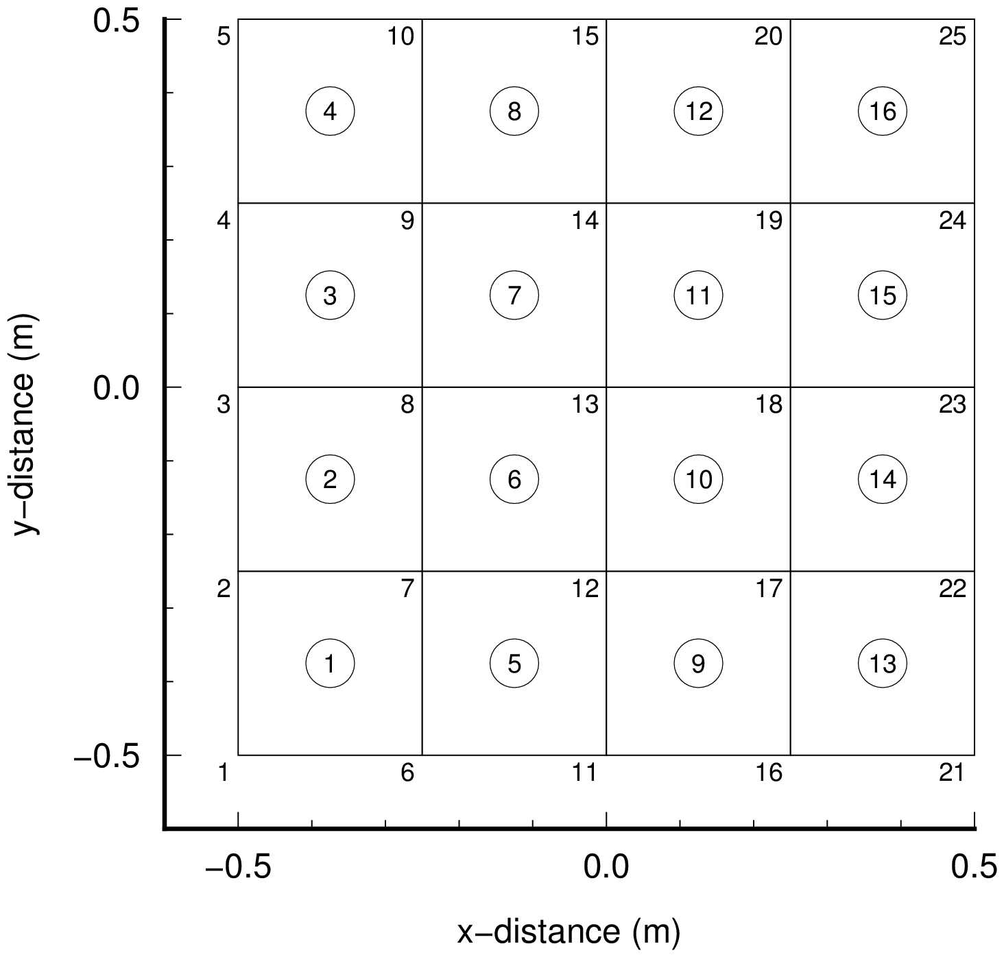
Adiabatic temperature raise model
Model has 4 side thermal insulation boundary. Initial temperature of domain is 20$^\circ$C and heat generation of elements are considered. 'delta' in the figure means time increment.
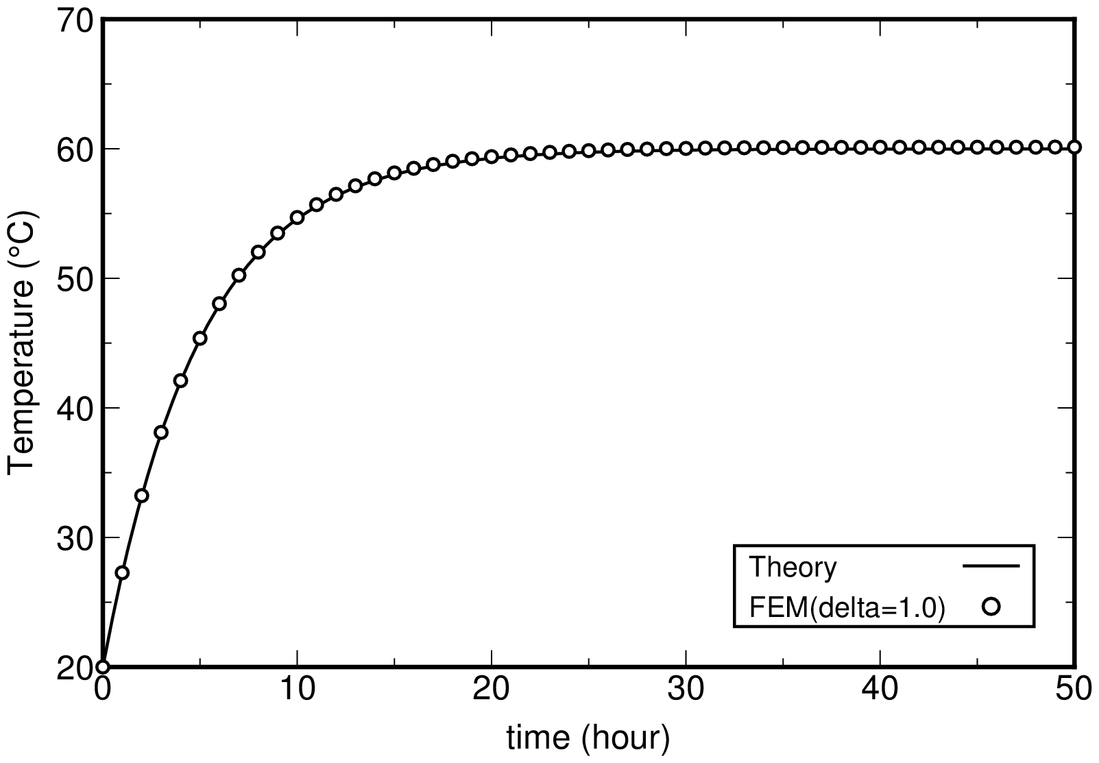 |
| Fig.2 Adiabatic temperature raise model (initial temperature: 20$^\circ$C) |
|---|
Given temperature boundary model
Time history analysis of temperature was carried out under following conditions.
| Conditions for Analysis | |
|---|---|
| Initial temperature of domain | 20$^\circ$C (for all area) |
| Temperature of top side | 40$^\circ$C (temperature change happens momentarily) |
| Temperature of bottom side | 0$^\circ$C (temperature change happens momentarily) |
| Left side and right side of domain | thermal insulation condition |
| heat generation of element | not considered |
| 'delta' in the figure means time increment. | |
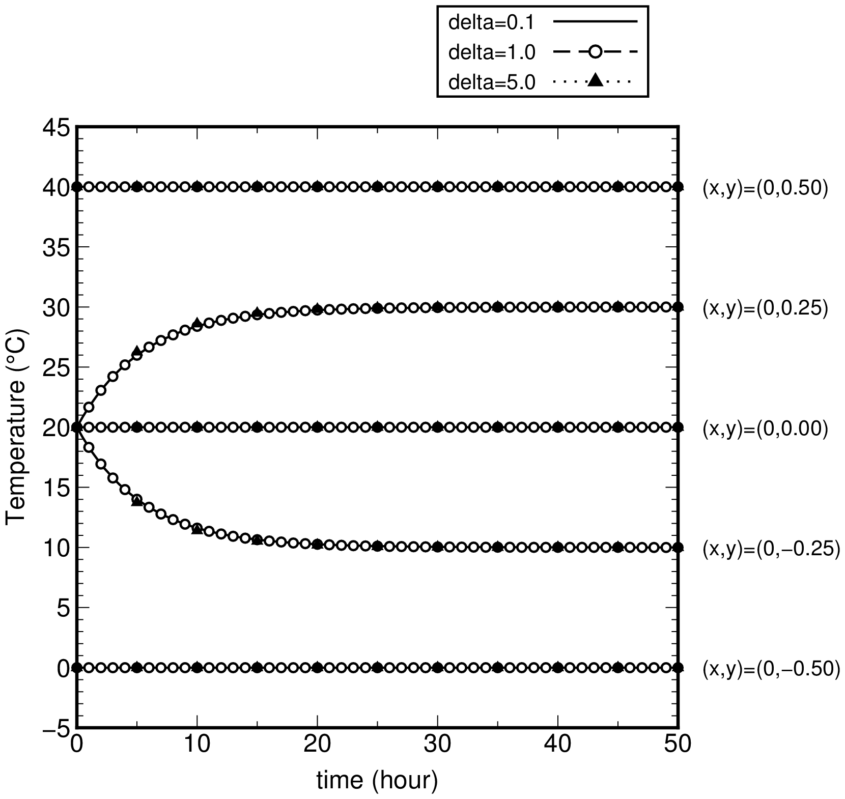 |
| Fig.3 Time history of temperature on given temperature boundary model
(Initial temperature: 10$^\circ$C, Top side: 40$^\circ$C, Bottom side: 0$^\circ$C) |
|---|
Heat transfer boundary model
Time history analysis of temperature was carried out under following conditions.
| Conditions for Analysis | |
|---|---|
| Initial temperature of domain | 20$^\circ$C (for all area) |
| Outside Temperature of domain | 10$^\circ$C |
| Boundary condition | 4 sides have heat transfer boundary for each |
| heat generation of element | considered |
| 'delta' in the figure means time increment. | |
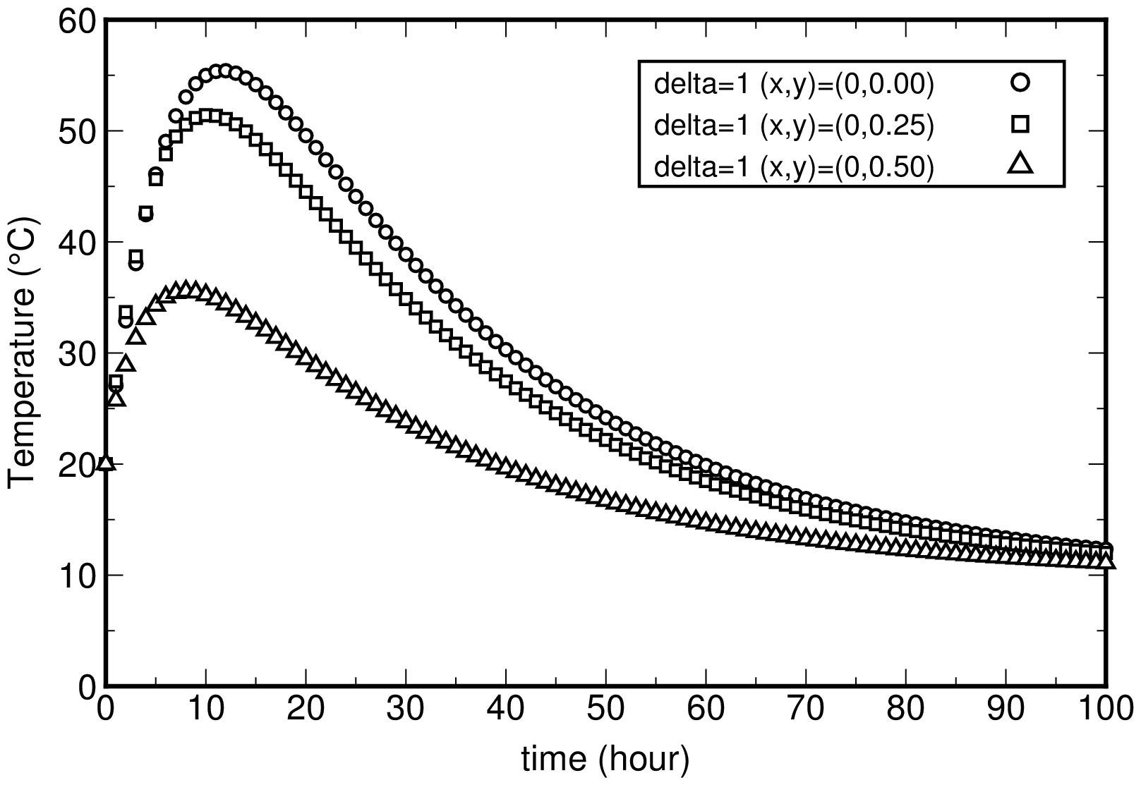 |
| Fig.4 Time history of temperature of the model with 4 heat transfer sides
(Initial temperature: 20$^\circ$C, Outside temperature: 10$^\circ$C) |
|---|
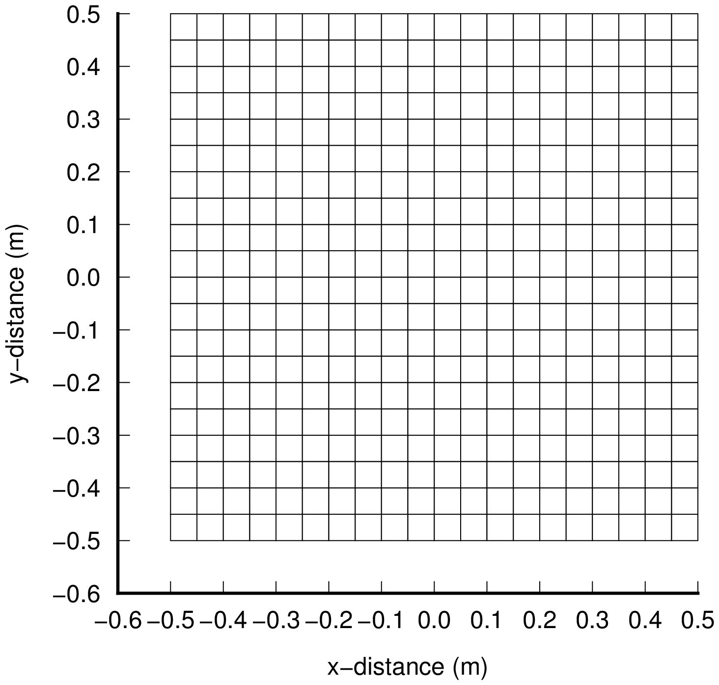
Model analysis with 400 elements
|
| ||||||||||||||||
Cleared matter by model analysis
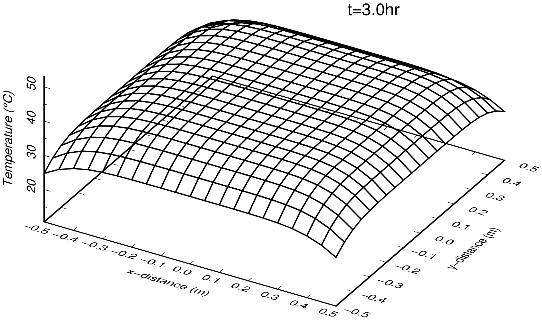
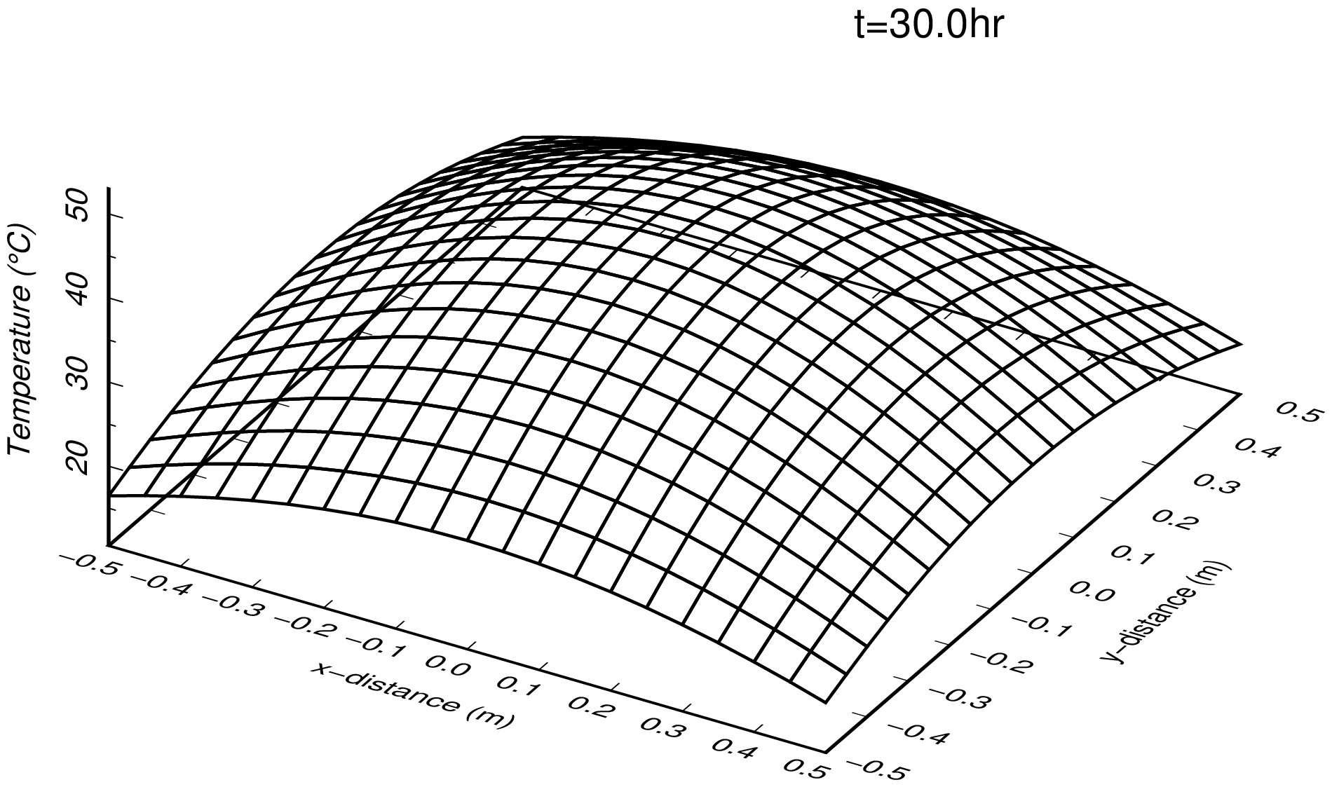
- In the case of rough element division, higher temperature will be obtained. (from comparison of Fig.4 and Fig.7)
- In the case of rough time increment, higher temperature will be obtained. (from Fig.7)
- In given temperature boundary model, the oscillating phenomenon of solution happens at the nodes near given temperature boundaries under the condition of fine element division and rough time increment. In this model, if fine element division is adopted to the model, it is necessary to adopt fine time increment in order to avoid the oscillating phenomenon of solution.(from Fig.3 and Fig.6)
- In heat transfer boundary model, the oscillating phenomenon of the solution resulting from the element division or time increment does not happen. (from Fig.4 and Fig.7)
Given temperature boundary model
Time history analysis of temperature was carried out under following conditions.
| Conditions for Analysis | |
|---|---|
| Initial temperature of domain | 20$^\circ$C (for all area) |
| Temperature of top side | 40$^\circ$C (temperature change happens momentarily) |
| Temperature of bottom side | 0$^\circ$C (temperature change happens momentarily) |
| Left side and right side of domain | thermal insulation condition |
| heat generation of element | not considered |
| 'delta' in the figure means time increment. | |
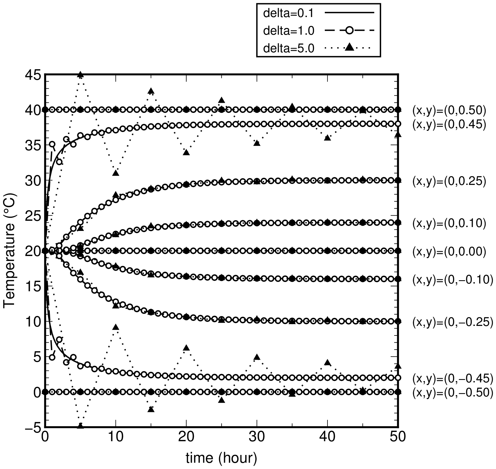 |
| Fig.6 Time history of temperature on given temperature boundary model
(Initial temperature: 10$^\circ$C, Top side: 40$^\circ$C, Bottom side: 0$^\circ$C) |
|---|
Heat transfer boundary model
Conditions of analysis and time history of temperature
Time history analysis of temperature was carried out under following conditions.
| Conditions for Analysis | |
|---|---|
| Initial temperature of domain | 20$^\circ$C (for all area) |
| Outside Temperature of domain | 10$^\circ$C |
| Boundary condition | 4 sides have heat transfer boundary for each |
| heat generation of element | considered |
| 'delta' in the figure means time increment. | |
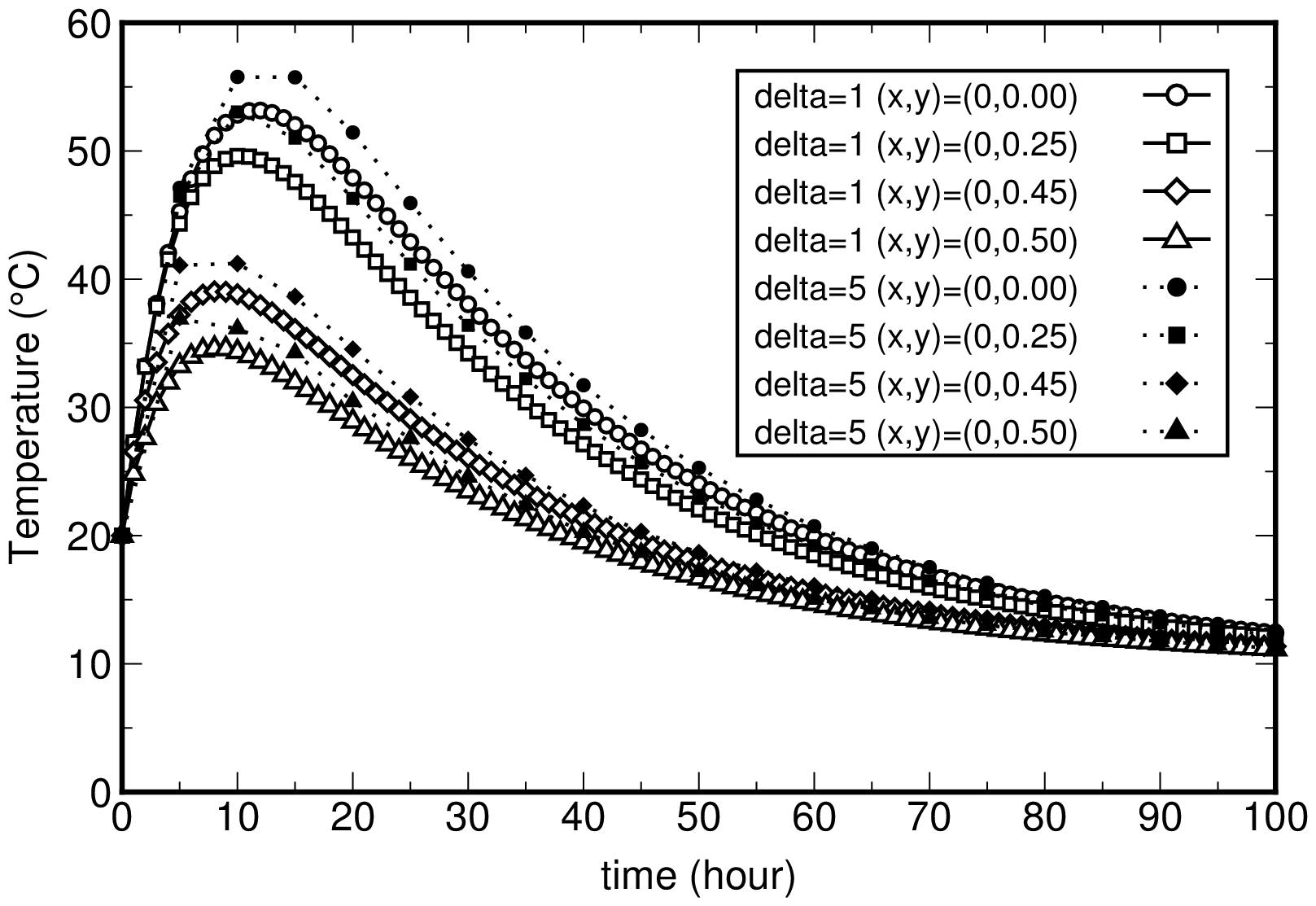 |
| Fig.7 Time history of temperature of the model with 4 heat transfer sides
(Initial temperature: 20$^\circ$C, Outside temperature: 10$^\circ$C) |
|---|
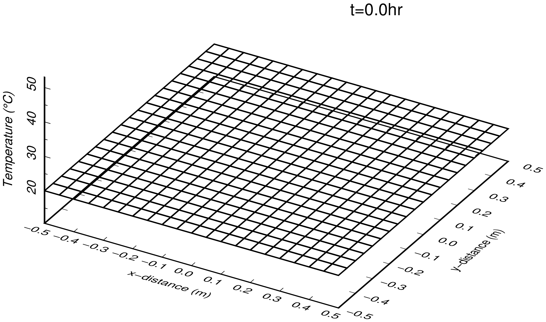
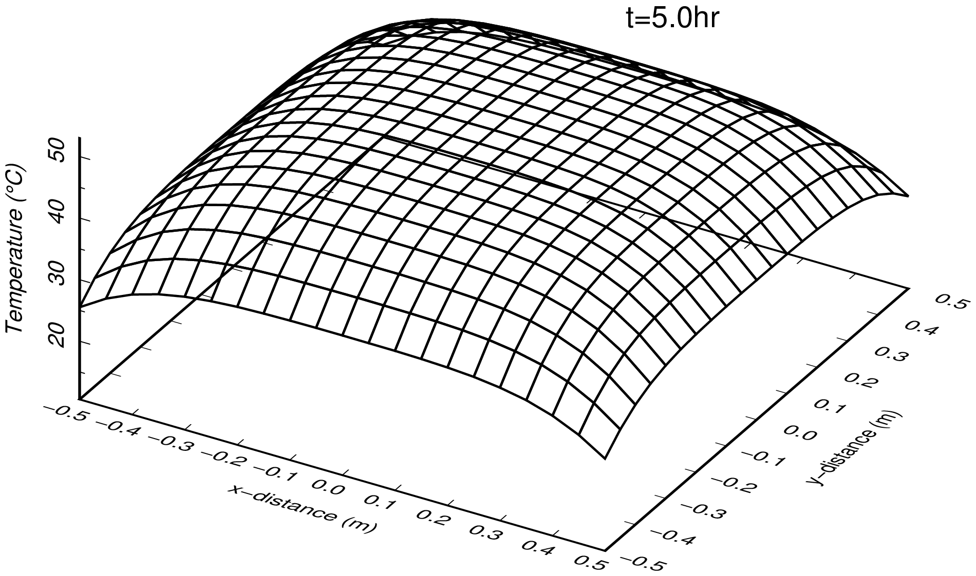
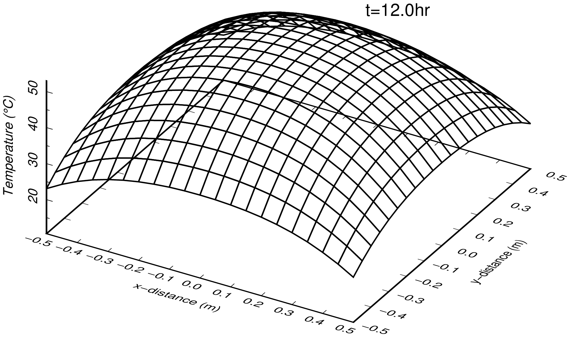
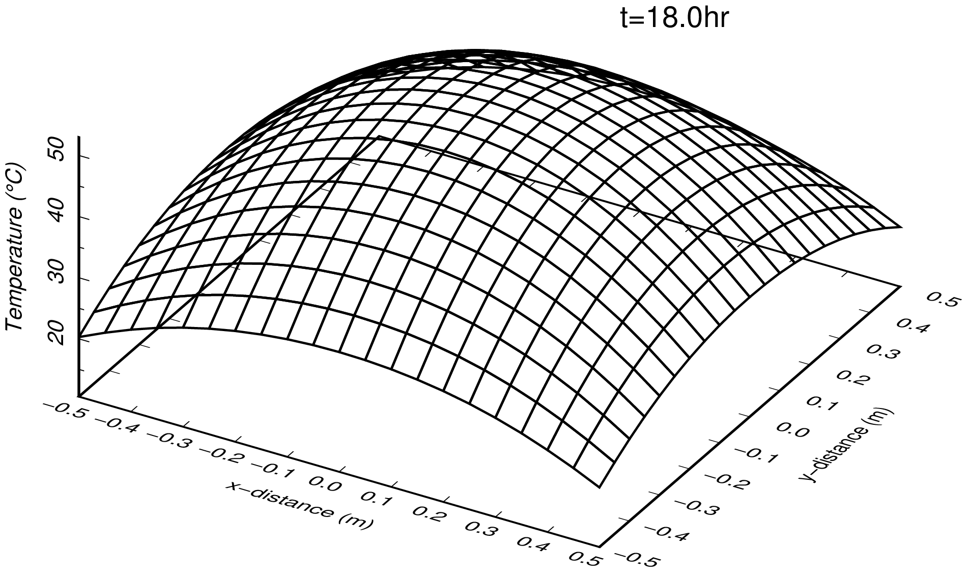
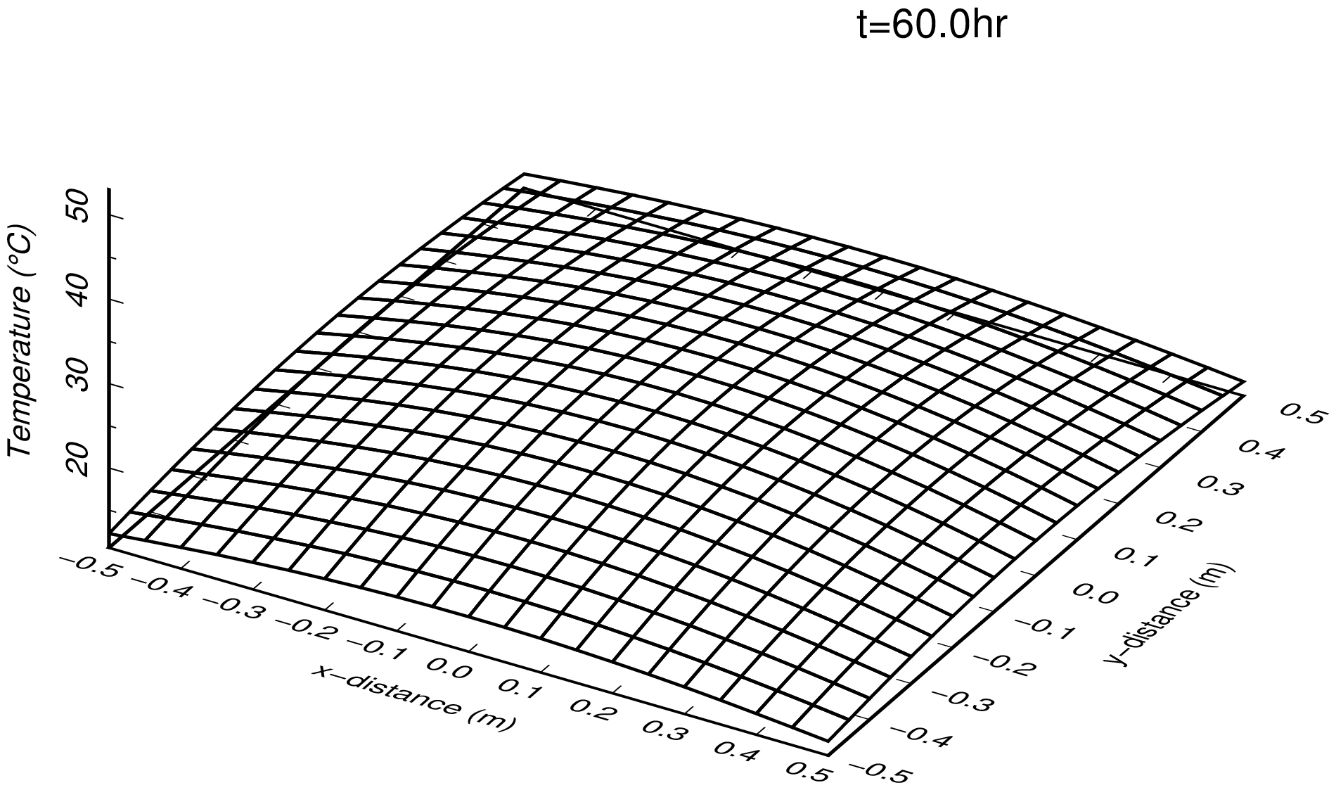
3D expression of temperature distribution
 |
 |
 |
 |
 |
 |
 |
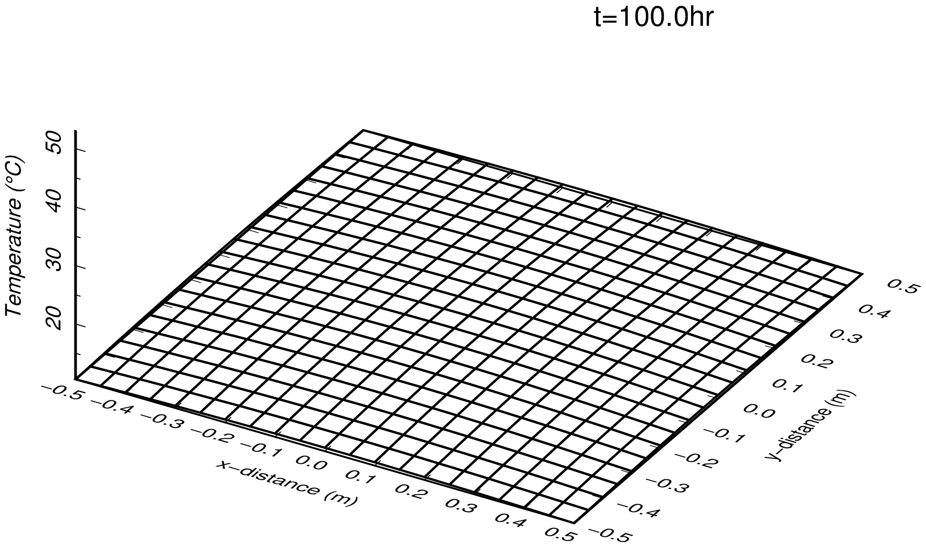 |
| Fig.8 Temperature distribution of heat transfer model (unit of 't': hour) | |
|---|---|
Programs and sample data
Fortran programs
| Filename | Description |
|---|---|
| f90_fem_heat.f90 | Unstedy het conduction analysis |
| f90_num_heat.f90 | Optimization of node number |
| f90_gmt_heat.f90 | Drawing program |
Shell scripts
| Filename | Description |
|---|---|
| a_fem_div4.txt | Shell script for execution of 16 elements model |
| a_fem_div20.txt | Shell script for execution of 400 elements model |
| a_draw_heat_small.txt | Drawing of 16 elements model |
| a_draw_heat_11_div20.txt | Drawing of 400 elements model |
| a_gra_test_div4.txt | GMT command for 16 elements model drawing |
| a_gra_11_div20.txt | GMT command for 400 elements model drawing (1) |
| a_gra_22_div20.txt | GMT command for 400 elements model drawing (2) |
Sample input data of 16 elements model
| Filename | Description |
|---|---|
| inp_test00_div4.csv | Sample data (adiabatic temperature raise) |
| inp_test11_div4.csv | Sample data (heat transfer) |
| inp_test22_div4_01.csv | Sample data (given temperature boundary: dt=0.1hr) |
| inp_test22_div4_10.csv | Sample data (given temperature boundary: dt=1.0hr) |
| inp_test22_div4_50.csv | Sample data (given temperature boundary: dt=5.0hr) |
| t_test00_div4.csv | Temperature data (adiabatic) |
| t_test11_div4.csv | Temperature data (heat transfer) |
| t_test22_div4.csv | Temperature data (given temperature) |
Sample input data of 400 elements model
| Filename | Description |
|---|---|
| inp_11_div20_01.csv | Original sample data (heat transfer: dt=0.1hr) |
| inp_11_div20_01m.csv | Optimized sample data (heat transfer: dt=0.1hr) |
| inp_11_div20_10.csv | Original sample data (heat transfer: dt=1.0hr) |
| inp_11_div20_10m.csv | Optimized sample data (heat transfer: dt=1.0hr) |
| inp_11_div20_50.csv | Original sample data (heat transfer: dt=5.0hr) |
| inp_11_div20_50m.csv | Optimized sample data (heat transfer: dt=5.0hr) |
| inp_22_div20_01.csv | Original sample data (given temperature: dt=0.1hr) |
| inp_22_div20_01m.csv | Optimized sample data (given temperature: dt=0.1hr) |
| inp_22_div20_10.csv | Original sample data (given temperature: dt=1.0hr) |
| inp_22_div20_10m.csv | Optimized sample data (given temperature: dt=1.0hr) |
| inp_22_div20_50.csv | Original sample data (given temperature: dt=5.0hr) |
| inp_22_div20_50m.csv | Optimized sample data (given temperature: dt=5.0hr) |
| t_11_div20.csv | Temperature data (heat transfer) |
| t_22_div20.csv | Temperature data (given temperature) |
Expression of the result of heat conduction analysis (f90_gmt_heat.f90)
Outline
This is a Fortran program to show FEM mesh and 3D plot of temperature distribution by using GMT.
Some explanations are shown below.
- This program shows 3D plot of temperature distribution by using the GMT command 'psxyz.'
- x-coordinate and y-coordinate are plane coordinate of elements, and z-coordinate is the temperature at defined time.
- Output filename is defined automatically in the program.
Following files must be prepared before execution of the program.
| Filename | Description | Remarks |
|---|---|---|
| _col_mesh.txt | Input file for defining mesh color. | Filename is fixed |
| _inp_base.txt | Input file for drawing information | Filename is fixed |
| fnameW.csv | Output file by FEM analysis | Filename is changeable |
Output file by FEM analysis is a output by the program 'f90_fem_heat' made by webmaster.
Description of Shell script
Shell script (a_draw_heat_11_div20.txt) which carries out the process is shown below. Some files which are read from Fortran program are made in this script.
001   gfortran -o f90_gmt_heat f90_gmt_heat.f90
002
003   # definition of mesh colour (1:MATEL)
004   echo 255,255,255 > _col_mesh.txt
005
006   # definition of basic data
007   # integer::ind,ibc
008   # real(4)::baselength,baseheight
009   # real(4)::bavx,bfvx
010   # real(4)::bavz,bfvz
011   # character::strx*100,stry*100
012   cat << EOT > _inp_base.txt
013   0 0
014   10.0 5.0
015   0.1 0.1
016   10 5
017   "x-distance (m)"
018   "y-distance (m)"
019   EOT
020
021   ./f90_gmt_heat out_11_div20_10m.csv
022   mv -f _fig_gmt_mesh.eps fig_gmt_mesh_div20.eps
023   for f in _fig_gmt_xyz_??.eps
024   do
025       mv -f $f ${f/_/}
026   done
027
028   rm _*
001
To compile the program of 'f90_gmt_heat.f90'
004
To make the file '_col_mesh.txt.' Mesh colors are defined by this file, 3 figures means 'R G B' in this file. In this example, new file is made using command 'echo' in this batch file, and since 1 material is used (parameter MATEL=1), 1 kind of color is defined.
012-019
To make the file '_inp_base.txt.' This file defines the parameters for GMT.
| ind | Draw node number and element number in FEM mesh. (0: no, 1: yes) |
| ibc | Draw boundary conditions in FEM mesh. (0: no, 1: yes) |
| baselength | Size of x and y-axis in unit of 'cm' |
| baseheight | Size of z-axis in unit of 'cm' |
| bavx | Value of 'a' in '-B' option for x and y-axis on GMT |
| bfvx | Value of 'f' in '-B' option for x and y-axis on GMT |
| bavz | Value of 'a' in '-B' option for z-axis on GMT |
| bfvz | Value of 'f' in '-B' option for z-axis on GMT |
| strx | Label for x-axis. Double prime (") is required because of character |
| stry | Label for y-axis. Double prime (") is required because of character |
Note) label for z-axis is fixed character 'Temperature.'
021
To execute the program 'f90_gmt_heat.' Functions of this execution file are to make GMT commands, to execute them and to make eps drawings.
Input file 'out_11_div20_10m.csv' which storages the result of FEM analysis is read from command line.
Output drawings are shown below.
| Filename | Description | Remarks |
|---|---|---|
| _fig_gmt_mesh.eps | FEM mesh drawing in eps format | Output filename is fixed. |
| _fig_gmt_xyz_xx.eps | 3D temperature distribution drawing in eps format | Output filename is fixed. 'xx' means time history. |
| Symbols for boundary conditions in FEM mesh drawing | |
|---|---|
| Symbol | Description |
| ○ | Boundary of given temperature |
| △ | Boundary of heat transfer side |
022-26
Rename of output eps files.
028
To delete work files