Outline of a program 'f90_fem_gfrm.f90'
- This is a program for Geometrically Nonlinear Analysis of 2D-Frame, and large displacement of elastic frame members can be simulated.
- Incremental Arc-Length Method is used to solve the incremental stiffness equations.
- Internal forces of the frame members are calculated using the linear stiffness matrix and the displacements without rigid body displacement.
- Simultaneous equations which has been linearized by incremental method are solved using Gauss-Jordan elimination. Because the dimension of matrix is not so large and the stiffness matrix sometimes becomes negative-definite.
- Input/Output file name can be defined arbitrarily with the format of 'csv' and those are inputted from command line of a terminal.
- Used language for program is 'Fortran 90' and used compiler is 'GNU gfortran.'
- Please note that it is assumed the directions of external loads don't change before and after deformation.
| Workable condition | |
|---|---|
| Item | Description |
| Element | 2D beam element. Geometrically Nonlinear behavior of a frame can be simulated. |
| Load | Specify the loaded nodes and load values |
| Displacement | Specify the nodes which are completely fixed. Only zero displacement can be considered. |
Incremental stiffness equation
\begin{equation*} \{\Delta f\}=[K_T]\{\Delta u\} \qquad [K_T]=[K_L]+[K_G] \end{equation*} \begin{align*} &\{\Delta f\}=\begin{Bmatrix} \Delta N_i & \Delta S_i & \Delta M_i & \Delta N_j & \Delta S_j & \Delta M_j \end{Bmatrix}^T \\ &\{\Delta u\}=\begin{Bmatrix} \Delta u_i & \Delta v_i & \Delta \theta_i & \Delta u_j & \Delta v_j & \Delta \theta_j \end{Bmatrix}^T \end{align*} \begin{align*} &[K_L]= \begin{bmatrix} EA/\ell & 0 & 0 & -EA/\ell & 0 & 0 \\ 0 & 12EI/\ell^3 & 6EI/\ell^2 & 0 & -12EI/\ell^3 & 6EI/\ell^2 \\ 0 & 6EI/\ell^2 & 4EI/\ell & 0 & -6EI/\ell^2 & 2EI/\ell \\ -EA/\ell & 0 & 0 & EA/\ell & 0 & 0 \\ 0 & -12EI/\ell^3 & -6EI/\ell^2 & 0 & 12EI/\ell^3 & -6EI/\ell^2 \\ 0 & 6EI/\ell^2 & 2EI/\ell & 0 & -6EI/\ell^2 & 4EI/\ell \end{bmatrix} \\ &[K_G]=P\cdot \begin{bmatrix} 1/\ell & 0 & 0 & -1/\ell & 0 & 0 \\ 0 & 6/5\ell & 1/10 & 0 & -6/5\ell & 1/10 \\ 0 & 1/10 & 2\ell/15 & 0 & -1/10 & -\ell/30 \\ -1/\ell & 0 & 0 & 1/\ell & 0 & 0 \\ 0 & -6/5\ell & -1/10 & 0 & 6/5\ell & -1/10 \\ 0 & 1/10 & -\ell/30 & 0 & -1/10 & 2\ell/15 \end{bmatrix} \end{align*}| $[K_T]$ | : Tangential stiffness matrix of an element |
| $[K_L]$ | : Linear stiffness matrix of an element |
| $[K_G]$ | : Geometrical non-linear stiffness matrix of an element |
| $P$ | : Axial force of an element (positive sign means tension) |
| $\{\Delta f\}$ | :Incremental equivalent nodal force vector of an element |
| $\{\Delta u\}$ | :Inclemental displacement vector of an element |
| $E , A , I , \ell$ | : Elastic modulus, section area, moment of inertia, element length |
| $\Delta N , \Delta S , \Delta M$ | : Increments of axial force, shear force and bending moment |
| $\Delta u , \Delta v , \Delta \theta$ | : Increments of displacements in axial direction, transverse direction and rotation |
| Subscripts $i$ and $j$ | : variables for node $i$ and node $j$ |
Calculation formulas for Internal forces
Calculation of internal force
The increments of internal force $\{\Delta r\}$ van be obtained using $[K_L]$ and $\{\Delta u^*\}$.
Where, $[K_L]$ is a linear stiffness matrix of an element,
and $\{\Delta u^*\}$ is an incremental displacement vector ecluding rigid rotation in local coordinate system.
\begin{equation*}
\{\Delta r\}=[K_L]\{\Delta u^*\}
\end{equation*}
\begin{align*}
&\{\Delta r\} =\begin{Bmatrix} \Delta N^*_i & \Delta S^*_i & \Delta M^*_i & \Delta N^*_j & \Delta S^*_j & \Delta M^*_j \end{Bmatrix}^T \\
&\{\Delta u^*\}=\begin{Bmatrix} \Delta u^*_i & \Delta v^*_i & \Delta \theta^*_i & \Delta u^*_j & \Delta v^*_j & \Delta \theta^*_j \end{Bmatrix}^T
\end{align*}
\begin{align*}
&\Delta u^*_i=0 &~& \Delta v^*_i=0 &~& \Delta \theta^*_i=(\tan\theta^*_i)_k-(\tan\theta^*_i)_{k-1} \\
&\Delta u^*_j=\Delta\ell & & \Delta v^*_j=0 & & \Delta \theta^*_j=(\tan\theta^*_j)_k-(\tan\theta^*_j)_{k-1}
\end{align*}
Where, $\Delta\ell$ means the difference of the previous element length and current element length. Regarding the rotation component, it is taken as the difference of the previous rotation angle (subscript $k-1$) and current rotation angle (subscript $k$).
Elimination of rigid rotation
The method of elimination of rigid rotation is shown below:
Using the addition formula for tangent,
\begin{align*} &\frac{dv^*}{dx^*}|_i=\tan\theta^*_i=\tan(\theta_i-R)=\frac{\tan\theta_i-\tan R}{1+\tan\theta_i\tan R} =\frac{(\ell+u_j-u_i)\tan\theta_i-(v_j-v_i)}{(\ell+u_j-u_i)+(v_j-v_i)\tan\theta_i} \\ &\frac{dv^*}{dx^*}|_j=\tan\theta^*_j=\tan(\theta_j-R)=\frac{\tan\theta_j-\tan R}{1+\tan\theta_j\tan R} =\frac{(\ell+u_j-u_i)\tan\theta_j-(v_j-v_i)}{(\ell+u_j-u_i)+(v_j-v_i)\tan\theta_j} \\ &\left(\tan R=\frac{v_j-v_i}{\ell+u_j-u_i}, \quad \frac{dv}{dx}|_i=\tan\theta_i, \quad \frac{dv}{dx}|_j=\tan\theta_j \right) \end{align*} |
| Elimination of rigid rotation |
|---|
Arc-Length Method
When simplified scalar load-displacement curve is considered, following equations can be obtained reffering below figure.
\begin{align*} K_T\cdot\Delta U=&\Delta\lambda\cdot\Delta F+\Delta R \\ \Delta U=&\Delta\lambda\cdot\Delta U_0+\Delta U_R \end{align*} \begin{align*} (\Delta s)^2&=(\Delta U)^2+(\Delta\lambda\cdot\phi\Delta F)^2 \\ &=(\Delta\lambda)^2\{(\Delta U_0)^2+(\phi\Delta F)^2\}+2\lambda\cdot(\Delta U_0\cdot\Delta U_R)+(\Delta U_R)^2 \end{align*} \begin{equation*} \Delta\lambda=\cfrac{-(\Delta U_0\cdot\Delta U_R)\pm\sqrt{\left\{(\Delta U_0)^2+(\phi\Delta F)^2)\right\}\cdot(\Delta s)^2-(\phi\Delta F\cdot\Delta U_R)^2}}{(\Delta U_0)^2+(\phi\Delta F)^2} \end{equation*} |
| Concept of Arc-Length method |
|---|
| where, | $K_T$ | : Tangential stiffness | $\Delta\lambda$ | : Coefficient for external force |
| $\Delta F$ | : External force increment | $\Delta U_0$ | : Displacement increment for external force | |
| $\Delta R$ | : Unbalanced force increment | $\Delta U_R$ | : Displacement increment for unbalanced | |
| $\Delta U$ | : Displacement increment | $\Delta s$ | : Arc length | |
| $\phi$ | : Scaling parameter |
Initial value of $\Delta\lambda$
If $\Delta U_R=0$ is assumed, initial value of $\Delta\lambda$ can be obtained as following equation.
\begin{equation*} \Delta\lambda_0=\pm\sqrt{\frac{(\Delta s)^2}{(\Delta U_0)^2+(\phi\Delta F)^2}} \end{equation*}Above equation can take two values, and it should be noted that a sign of $\Delta\lambda_0$ is very important in Arc-Length method.
A sign of $\Delta\lambda_0$ is defined as shown below:
- Define a displacement increment vector ${\Delta U_{-1}}$ from previous equilibrium point to current equilibrium point.
- Calculate ${\Delta U_0}$ as ${\Delta U_0}=[K_T]^{-1}{\Delta F}$.
- Calculate an inner product ${\Delta U_{-1}}^T{\Delta U_0}=|\Delta U_{-1}|\cdot |\Delta U_0|\cdot \cos\theta$, where $\theta$ is an angle between 2 displacement increment vectors.
- If an inner product ${\Delta U_{-1}}^T{\Delta U_0} \geqq 0$, the angle $\theta$ is less than or equal to 90 degree. In this case, $\Delta\lambda_0$ has positive sign.
- If an inner product ${\Delta U_{-1}}^T{\Delta U_0} \lt 0$, the angle $\theta$ is greater than 90 degree. In this case, $\Delta\lambda_0$ has negative sign.
Regarding the scaling parameter $\phi$, it can be obtained as following equation. In this program, recommended value of $\alpha$ is one ($\alpha=1.0$). \begin{equation*} \phi=\sqrt{\frac{\alpha}{\{\Delta F\}^T\{\Delta F\}}} \end{equation*}
Regarding the arc length $\Delta s$, it can be obtained assuming $\Delta\lambda=1.0$.
\begin{equation*} \Delta s=\sqrt{\{\Delta U_0\}^T\{\Delta U_0\}+\phi^2\cdot\{\Delta F\}^T\{\Delta F\}} \qquad (\Delta\lambda_0=1.0) \end{equation*}Correction factor $\Delta\lambda$ for iterative calculation
Referring above conceptial figure and replacing $\Delta s$ to $\Delta L$, following equation can be obtained.
\begin{align*} (\Delta L)^2&=(\Delta U)^2+(\Delta\lambda\cdot\phi\Delta F)^2 \\ &=(\Delta\lambda)^2\{(\Delta U_0)^2+(\phi\Delta F)^2\}+2\Delta\lambda\cdot(\Delta U_0\cdot\Delta U_R)+(\Delta U_R)^2 \end{align*}From the condition of minimization of $(\Delta L)^2$, $\Delta\lambda$ can be calculate as following equation.
\begin{equation*} \frac{d(\Delta L)^2}{d\Delta\lambda}=0 \quad\rightarrow\quad \Delta\lambda=-\frac{\Delta U_0\cdot\Delta U_R}{(\Delta U_0)^2+(\phi\Delta F)^2} \end{equation*}Flowchart for analysis
| $\{F\}$ | : Total external force vector at equilibrium point |
| $\{\Delta F\}$ | : External incremental force vector |
| $\{R\}$ | : Internal force vector |
| $\{\Delta R\}$ | : Unbalanced force vector |
| $\{U\}$ | : Total displacement vector |
| $\{\Delta U\}$ | : Displacement increment vector |
| $\{\Delta U_0\}$ | : Displacement increment vector for external force increment |
| $\{\Delta U_R\}$ | : Displacement increment vector for unbalanced force |
| $\{\Delta U_{-1}\}$ | : Displacement increment vector from previous equilibrium point to current equilibrium point |
| $[K_T]$ | : Tangential stiffness matrix including non-linear component |
| $\Delta s$ | : Arc length |
| $\lambda$ | : Coefficient for external force increment and displacement increment |
| $\Delta\lambda$ | : Increment of coefficient $\lambda$ |
| $\phi$ | : Scaling parameter |
 |
| Flowchart of Calculation |
|---|
Input data from command line
./f90_fem_gfrm fnameR fnameW nlmax itmax coefA
| f90_fem_gfrm | Compiled program |
| fnameR | Input filename |
| fnameW | Output file name |
| nlmax | Limit of Loading steps |
| itmax | Limit of Iteration steps |
| coef | Scaling parameter for Incremental Arc-Lemgth method |
Format of input data file ('csv' format)
Comment                         # Comments
NODT,NELT,MATEL,KOX,KOY,KOZ,NF  # Basic values for analysis
Em,AA,AI                        # material properties
    ....(1 to MATEL)....        #
node-1,node-2,matno             # Element connectivity, material set number
    ....(1 to NELT)....         #
x,y                             # Node coordinates
    ....(1 to NODT)....         #
nokx                            # Fixed node number in x-direction
    ....(1 to KOX)....          # (Omit data input if KOX=0)
noky                            # Fixed node number in y-direction
    ....(1 to KOY)....          # (Omit data input if KOY=0)
nokz                            # Fixed node number in rotation
    ....(1 to KOZ)....          # (Omit data input if KOZ=0)
node,dfx,dfy,dfz                # loaded node number, Load increments in x & y-direction, Moment value
    ....(1 to NF)....           # (Omit data input if NF=0)
| NODT | : Number of nodes | Em | : Elastic modulus of element |
| NELT | : Number of elements | AA | : Section area of element |
| MATEL | : Number of material sets | AI | : Moment of inertia of element |
| KOX | : Number of fixed nodes in x-direction | matno | : Material set number |
| KOY | : Number of fixed nodes in y-direction | ||
| KOZ | : Number of fixed nodes in rotation | ||
| NF | : Number of loaded nodes | ||
Notice
- Fixed node means the node which is restricted completely.
- Since stress resultants of element are defined as equivalent nodal forces in local coordinate system, it is necessary to note that signs are different from it on general structural mechanics. Positive directions are always right-direction, upward-direction and counterclockwise direction for each node in local coordinate system.
Format of output file ('csv' format)
Comment
NODT,NELT,MATEL,KOX,KOY,KOZ,NF,nlmax,itmax
(Each value for above item)
*node characteristics
node,x,y,dfx,dfy,dfz,fix-x,fix-y,fix-z
    node     : Node number
    x,y      : x & y-coordinates
    dfx,dfy,dfz : Nodal forces in x & y direction and Moment of node
    fix-x    : x-direction restricted condition (1: restricted, 0: not restricted)
    fix-y    : y-direction restricted condition (1: restricted, 0: not restricted)
    fix-z    : Restricted condition for rotation (1: restricted, 0: not restricted)
  .....(1 to NODT).....
*element characteristics
element,node-1,node-2,E,A,I,matno
    element       : Element number
    node-1,node-2 : Element-nodes relationship
    E             : Elastic modulus of element
    A             : Section area of element
    I             : Moment of inertia of element
    matno         : Material set number
  .....(1 to NELT).....
*** New load step ***
nload,iteration,lam,deltaS,coefA
(Each value for above item)
*displacements and forces
node,coord-x,coord-y,dist-x,dist-y,dist-z,ff-x,ff-y,ff-z,ftvec-x,ftvec-y,ftvec-z
    node                    : Node number
    coord-x,coord-y         : Coordinates in x & y-directions
    dist-x,dist-y,dist-z    : Nodal displacements in x & y & rotation directions
    ff-x,ff-y,ff-z          : External loads in x & y & rotation directions
    ftvec-x,ftvec-y,ftvec-z : Unbalanced forces in x & y & rotation directions
  .....(1 to NODT).....
*stress resultants
element,Ni,Si,Mi,Nj,Sj,Mj
    element : Element number
    Ni,Nj   : Axial forces at node 'i' and 'j'
    Si,Sj   : Shear forces at node 'i' and 'j'
    Mi,Mj   : Moments at node 'i' and 'j'
  .....(1 to NELT).....
*** New load step ***
.....
=== (1 to nlmax) ===
.....
NODT=(Number of nodes) nt=(nt) mm=(mm)
Calculation time=(calculation time)
Date_time=(date of execution)
    nt : Total degrees of freedom of FE equation
    mm : Dimension of reduced FE equation
Sample drawings
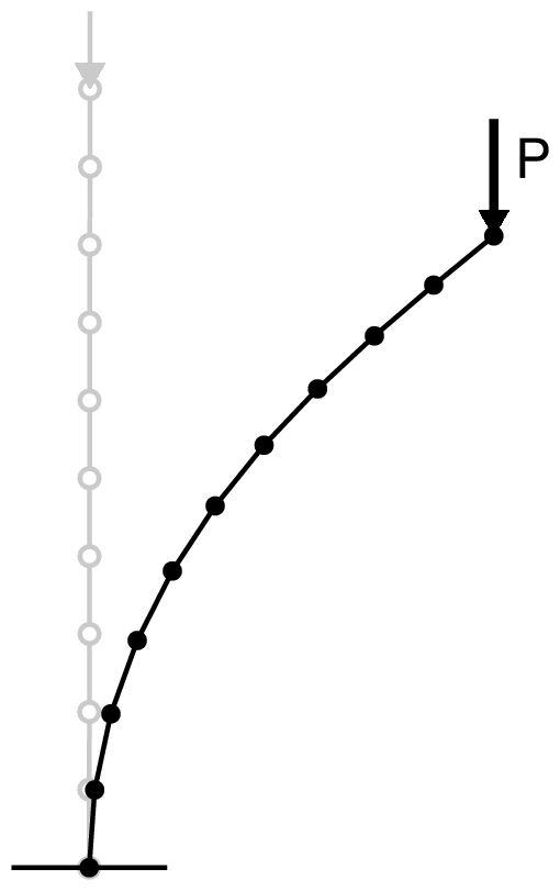
Elastica
| L=1,000 mm |
| E=200,000 N/mm$^2$ |
| A=100 mm$^2$ |
| I=833 mm$^4$ |
| Initial deflection v$_0$=1 mm (cosine curve) |
| Buckling load Pcr=$\pi^2$ EI / 4 L$^2$=411.07 N |
 |
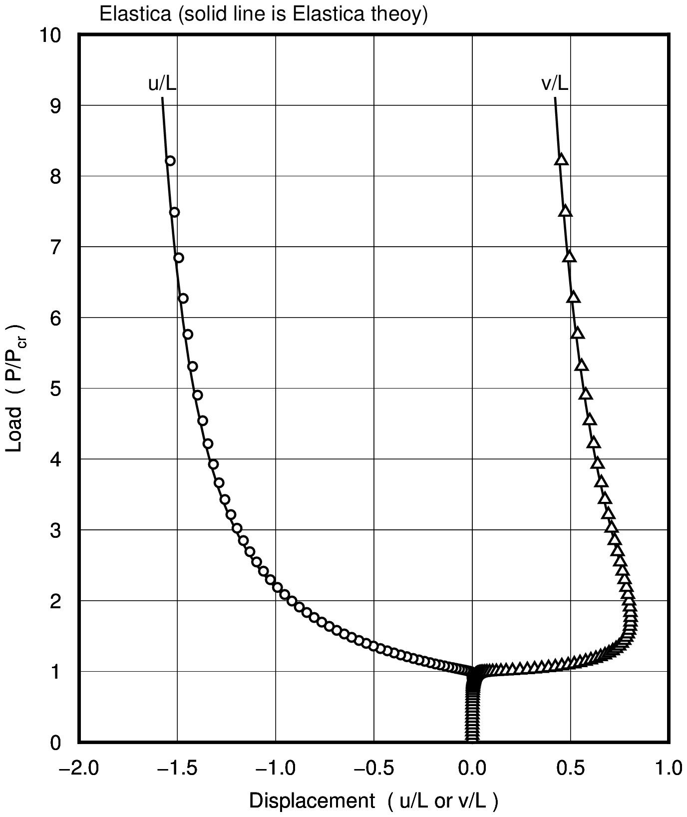 |
| Elastica | |
|---|---|
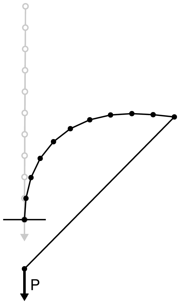
Column with Cable
| Column | Cable |
|---|---|
| L=1,000 mm | |
| E=200,000 N/mm$^2$ | E=200,000 N/mm$^2$ |
| A=100 mm$^2$ | A=28.3 mm$^2$ |
| I=833 mm$^4$ | |
| Initial deflection v$_0$=5 mm (cosine curve) | |
| Buckling Load Pcr=$\pi^2$ EI / L$^2$=1644.3 N | |
 |
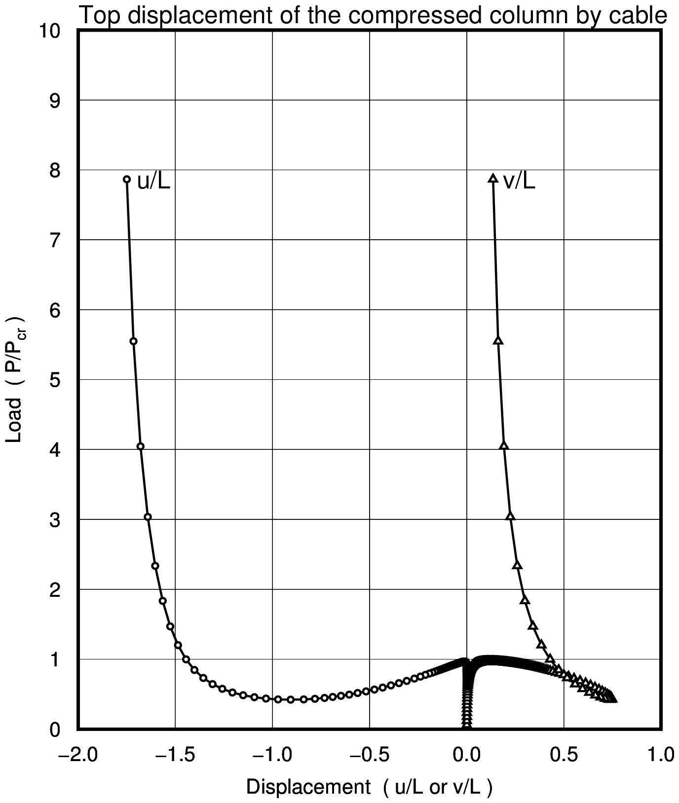 |
| Column with Cable | |
|---|---|
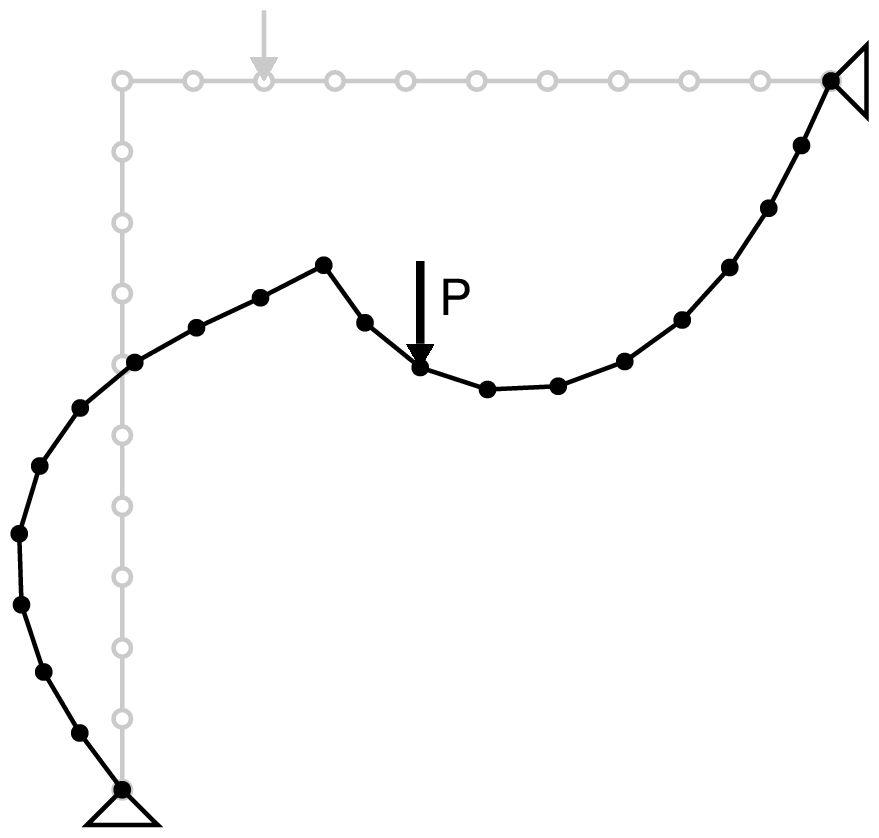
Lee's Frame
| L=1,000 mm |
| E=200,000 N/mm$^2$ |
| A=100 mm$^2$ |
| I=833 mm$^4$ |
 |
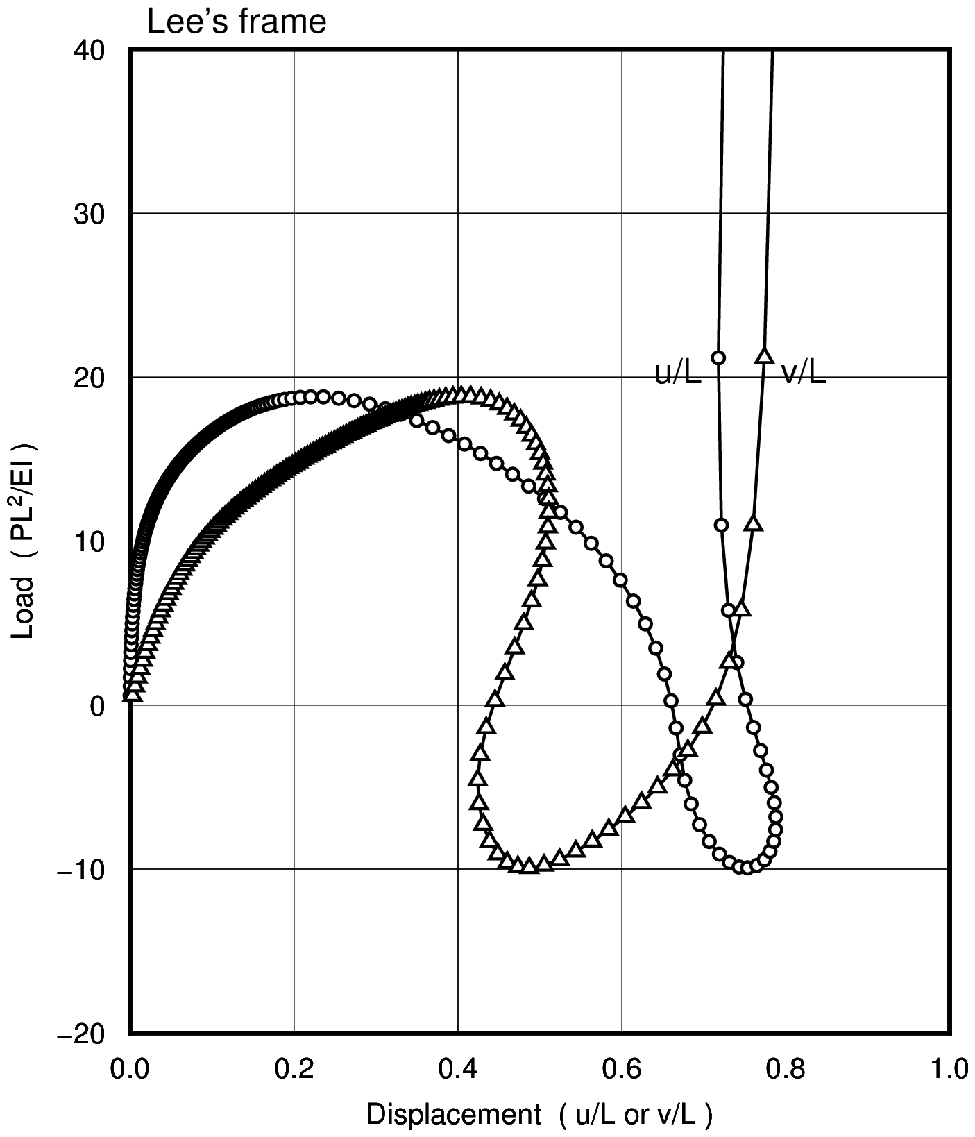 |
| Lee's Frame | |
|---|---|
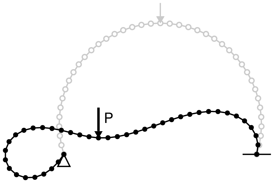
Arch with hinge and fixed support
| R=500 mm |
| Center Angle=215$^\circ$ |
| E=200,000 N/mm$^2$ |
| A=100 mm$^2$ |
| I=833 mm$^4$ |
 |
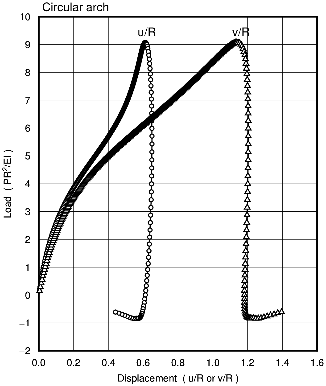 |
| Arch with hinge and fixed support | |
|---|---|
Programs and sample data
Fortran programs
| Filename | Description |
|---|---|
| f90_fem_gfrm.f90 | Geometrically Non-linear Analysis of 2D frame |
| f90_fig_gfrm.f90 | Drawing |
| f90_elas.f90 | Elastica Theory |
Example of usage of program 'f90_fig_gfrm.f90'
gfortran -o f90_fig_gfrm.exe f90_fig_gfrm.f90
f90_fig_gfrm.exe out_lee.csv _dat_lee.csv 13 2 13
In above commands,
- First figure 13 means node number of which you want to plot a load
- Second figure 2 means number of freedom of load. 1: x-direction, 2: y-direction, 3: z-direction
- Third figure 13 means node number of which you want to plot deflections.
In a file '_dat_lee.csv',
- First column: load at node 13 in y-direction
- Second column: deflection at node 13 in x-direction
- Third column: deflection at node 13 in y-direction
After above, if you use gnuplot, you can get a drawing using following procedure. (following is for mac)
kk@my-mac ~/DATA/Fortran/dir_fem_gfrm $ gnuplot

G N U P L O T
Version 5.0 patchlevel 1    last modified 2015-06-07

Copyright (C) 1986-1993, 1998, 2004, 2007-2015
Thomas Williams, Colin Kelley and many others

gnuplot home:     http://www.gnuplot.info
faq, bugs, etc:   type "help FAQ"
immediate help:   type "help"  (plot window: hit 'h')

Terminal type set to 'x11'
gnuplot> L=1000
gnuplot> E=200000
gnuplot> I=833
gnuplot> set xrange [0:1]
gnuplot> set yrange [-20:40]
gnuplot> set datafile separator ","
gnuplot> plot '_dat_lee.csv' using ($2/L):(-$1*L*L/E/I) with lines
gnuplot>
Shell scripts
| Filename | Description |
|---|---|
| a_ctl.txt | Control |
| a_f90.txt | Execution of f90 program |
| a_fig.txt | Make drawing data |
| a_fig_elas.txt | GMT command for Displacement-Load curve (1) |
| a_fig_ccbc.txt | GMT command for Displacement-Load curve (2) |
| a_fig_lee.txt | GMT command for Displacement-Load curve (3) |
| a_fig_cdarch.txt | GMT command for Displacement-Load curve (4) |
| a_fig_mode.txt | GMT command for mode drawing |
Input data samples
| Filename | Description |
|---|---|
| inp_cl_10.csv | Input data sample (1) |
| inp_ccbc.csv | Input data sample (2) |
| inp_lee.csv | Input data sample (3) |
| inp_cdarch.csv | Input data sample (4) |
Calculation example of Frames with Semi-Rigid Connections
Programs and Document
| Filename | Description |
|---|---|
| f90_fem_m_1.f90 | Non-linear analysis program |
| f90_fig_gfrm.f90 | Load-displacement relationship pick up program |
| a_f90.txt | Execution program including data making |
| a_gpl_pd.txt | gnuplot command for Load-Displacement curves |
| a_gpl_ds.txt | gnuplot command for Load-$\Delta s$ curves |
| a_gpl.txt | gnuplot command for Critical load-Fixity Factor relationship |
| TeX_fem_semirigid.pdf | Theory and Calculation example |
References
- [1] Optimization of Frames with Semi-Rigid Connections, L.M.C.Simoes, Computers & Structures Vol.60, No.4, pp.531-539, 1996
- [2] Design of non-linear semi-rigid steel frames with semi-rigid column bases, S.O.Degertekin, M.S.Hayalioglu, Electronic Journal of Structural Engineering, 4 (2..4)
- [3] An Investigation for Semi-Rigid Frames by Different Connection Models, Ali Ugur Ozturk and Mutlu Secer, Mathematical and Computational Applications, Vol.10, No.1, pp.35-44, 2005
- [4] Computational procedures for nonlinear analysis of frames with semi-rigid connections, Leonardo Pinheiro and Ricardo A.M.Silveira, Latin America Journal of Solid and Structures, 2 (2005) 339-367
- [5] Nonlinear Analysis of Semi-Rigid Frames with Rigid and Sections, S.Seren Akavci, Iranian Journal of Science & Technology, Transaction B, Engineering, Vol.31, No.B5, pp567-571
(note)
The stiffnes matrices of beam with semi-rigid connections in the reference [1], [2] and the first type in reference [3] give same result, alyhough the expression of each stiffnes matrix is fifferent.