Equations for analysis
Storage Function Method is framed by following equations.
Basic equations
\begin{align} &\cfrac{dS}{dt}=r_e(t-T_L)-q_c(t) & \text{Equation of continuity}\\ &S(t)=k\cdot \{q_c(t)\}^p & \text{Relationship between Storage and Direct run-off}\\ &r_e(t)=f\cdot R(t) & \text{Effective rainfall} \end{align}| $S(t)$ | : Storage (mm/hr) | $k$ | : Constant for storage function |
| $r_e(t)$ | : Effective rainfall (mm/hr) | $p$ | : Constant for storage function |
| $T_L$ | : Delay time (hr) | $f$ | : Rate of flow (constant) |
| $q_c(t)$ | : Direct run-off (mm/hr) | $R(t)$ | : Observed rainfall (mm/hr) |
Equations for Direct run-off
\begin{align} &q_c(t)=q(t)-q_B(t) & \text{Direct run-off}\\ &q(t)=\cfrac{3.6\cdot Q(t)}{A} & \text{Total run-off}\\ &q_B(t)=q_1+(i-n_1)\cfrac{q_2-q_1}{n_2-n_1} & \text{Base run-off} \end{align}| $q_c(t)$ | : Direct run-off(mm/hr) | $Q(t)$ | : Observed discharge (m$^3$/s) | ||||||||||||
| $q_B(t)$ | : Base run-off(mm/hr) | $A$ | : Catchment area (km$^2$) | ||||||||||||
| $q(t)$ | : Total run-off(mm/hr) | ||||||||||||||
| $n_1$ | : Start point of direct run-off | $q_1$ | : Run-off at start point of direct run-off | ||||||||||||
| $n_2$ | : End point of direct run-off | $q_2$ | : Run-off at end point of direct run-off | ||||||||||||
| $i$ | : Integer from $n_1$ until $n_2$ | ||||||||||||||
| $f$ | : Rate of flow | $q_c$ | : Direct run-off (mm/hr) | $R_T$ | : Observed rainfall (mm/hr) |
where, observed rainfall means that it is shifted one for same times as the times counted direct run-off.
Estimation of parameters and reproduction of Hydrograph
Equation of continuity is approximated into following finite difference approximation.
\begin{equation} \cfrac{dS}{dt}=r_e(t-T_L)-q_c(t) \quad\Rightarrow\quad S(t+\Delta t)=S(t)+\Delta t\cdot r_e(t+\Delta t -T_L)-\cfrac{\Delta t}{2}\left\{q_c(t+\Delta t)+q_c(t)\right\} \end{equation}In above, since $q_c(t)$ and $r_e(t)$ are known for whole times, the values of $S(t)$ can be obtained successively by setting the initial value of $S(0)=0$ at $t=0$.
About delay time $T_L$, the proper value of it can be obtained by trial changing the value of $L_T$ from zero.
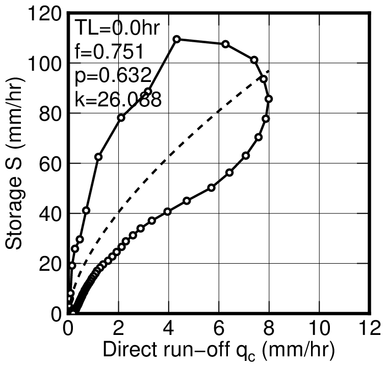
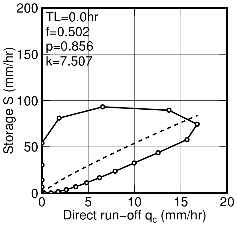
There is following relationship between storage $S$ and direct run-off $q_c$.
\begin{equation} S=k\cdot \{q_c\}^p \quad\Rightarrow\quad \ln S=\ln k+p\cdot \ln q_c \end{equation} <>pPractically, by comparison with the relations between the storage $S$ and direct run-off $q_c$ on log-log graph while changing $T_L$, the value of $T_L$ can be established when an agreement degree of the behavior is the highest during flow increase time and flow decrease time.The value of $k$ and $p$ can be obtained by a regression analysis on log-log graph using established $T_L$.
After obtaining the constant values of $k$, $p$ and $T_L$, the time history of $q_c$ can be obtained by the numerical integration of following differential equation using such as Runge-Kutta mathod.
\begin{equation} \cfrac{dq_c}{dt}=\cfrac{1}{k\cdot p}\cdot(r_e-q_c)\cdot q_c{}^{1-p} \end{equation}Where, the time history of $q_c$ in above equation is not related the values which were used for obtaining storage $S$. At this time, the values of $r_e$, $p$ and $k$ are known and the time history of $q_c$ is unknown. Therefore, it is necessary to set the small initial value of $q_c$ at the equivalent time of starting point of separation $n_1$. After this, the time history of $q_c$ can be calculated successively using numerical integration.
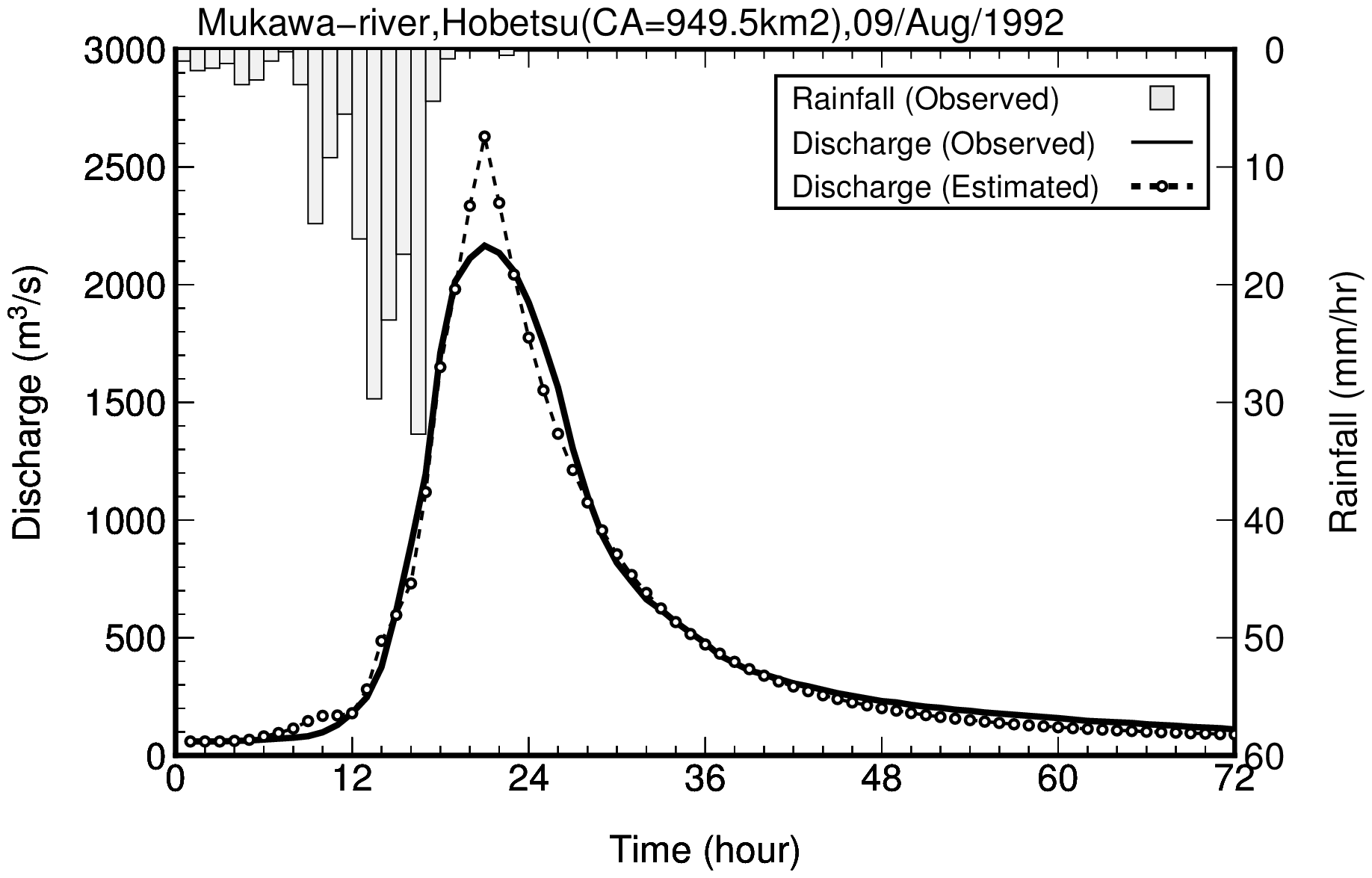
If the time history of $q_c$ can be known, Hydrograph can be re-producted using following equation.
\begin{equation} Q=\cfrac{1}{3.6}\cdot A \cdot (q_c+q_B) \end{equation}Where, please take care of units. The unit of discharge $Q$ is 'm$^3$/s', the unit for direct run-off $q_c$ and base run-off $q_B$ is 'mm/hr', the unit of catchment area is 'km$^2$'.
Examples of analysis
Trial calculation for following cases were done.
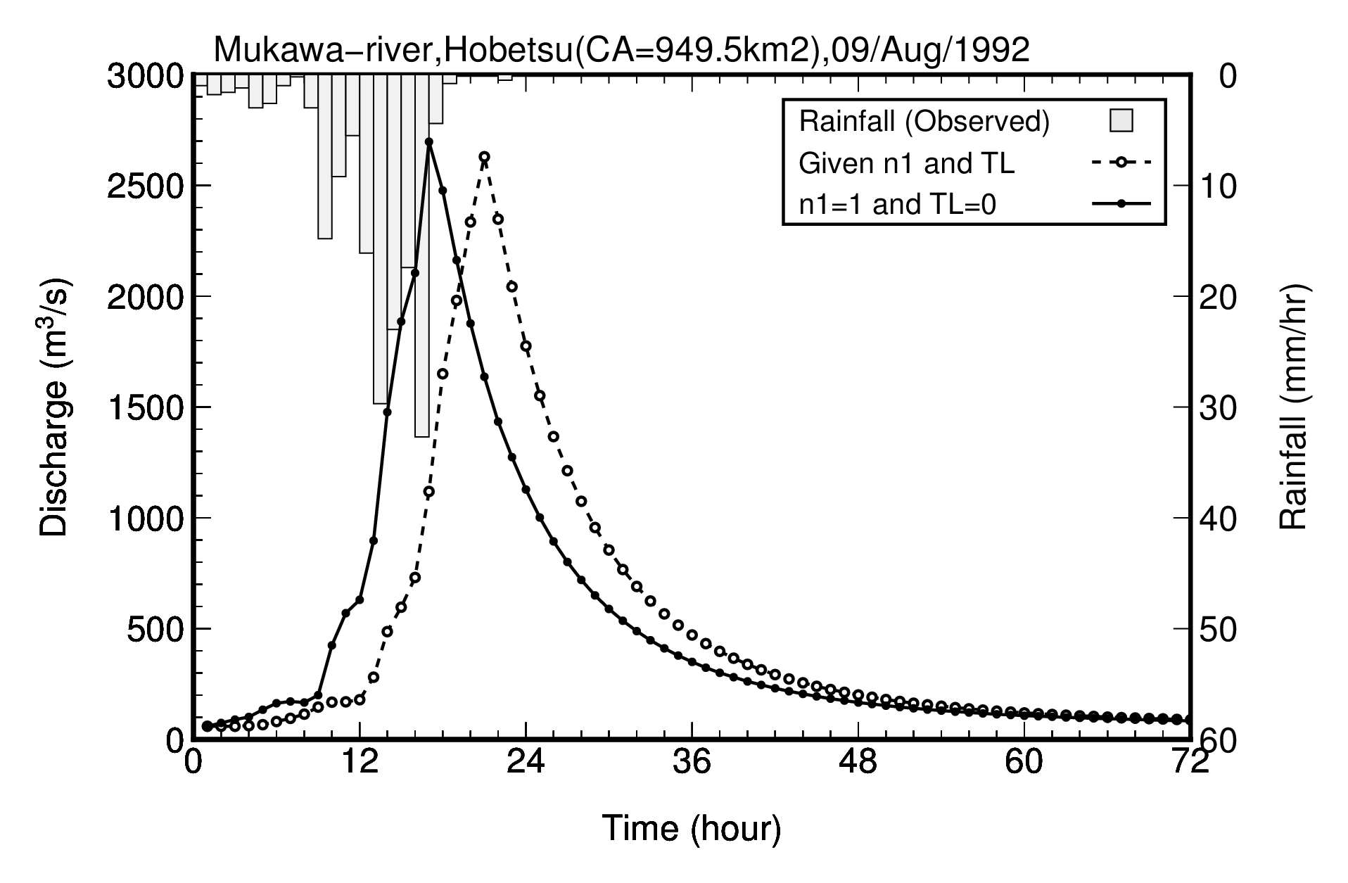
- Case 1 : Mukawa-river (09/Aug/1992)
(Source: 若手水文学研究会:現場のための水文学(1) -- 流出解析 その1 -- in Japanese character) - Case 2 : Sample data from textbook
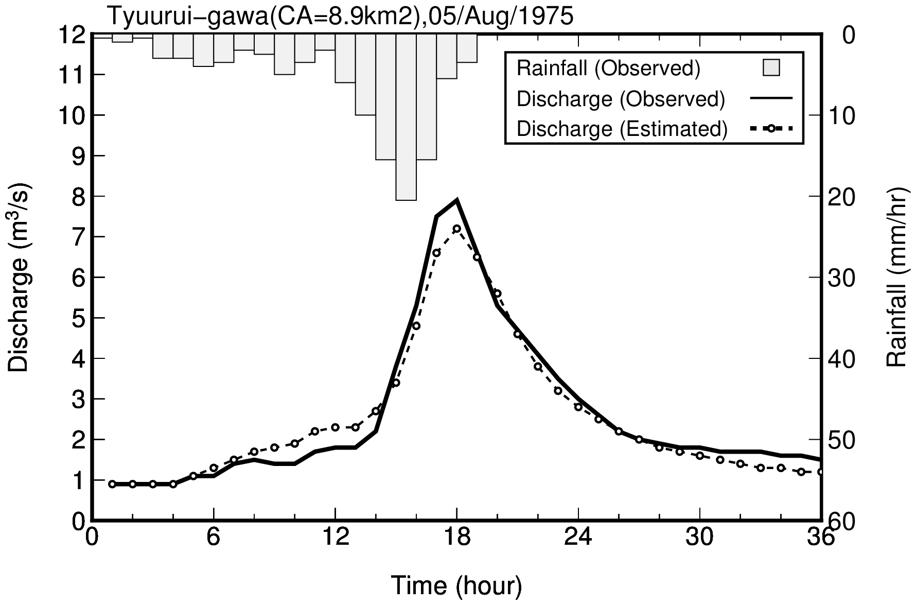
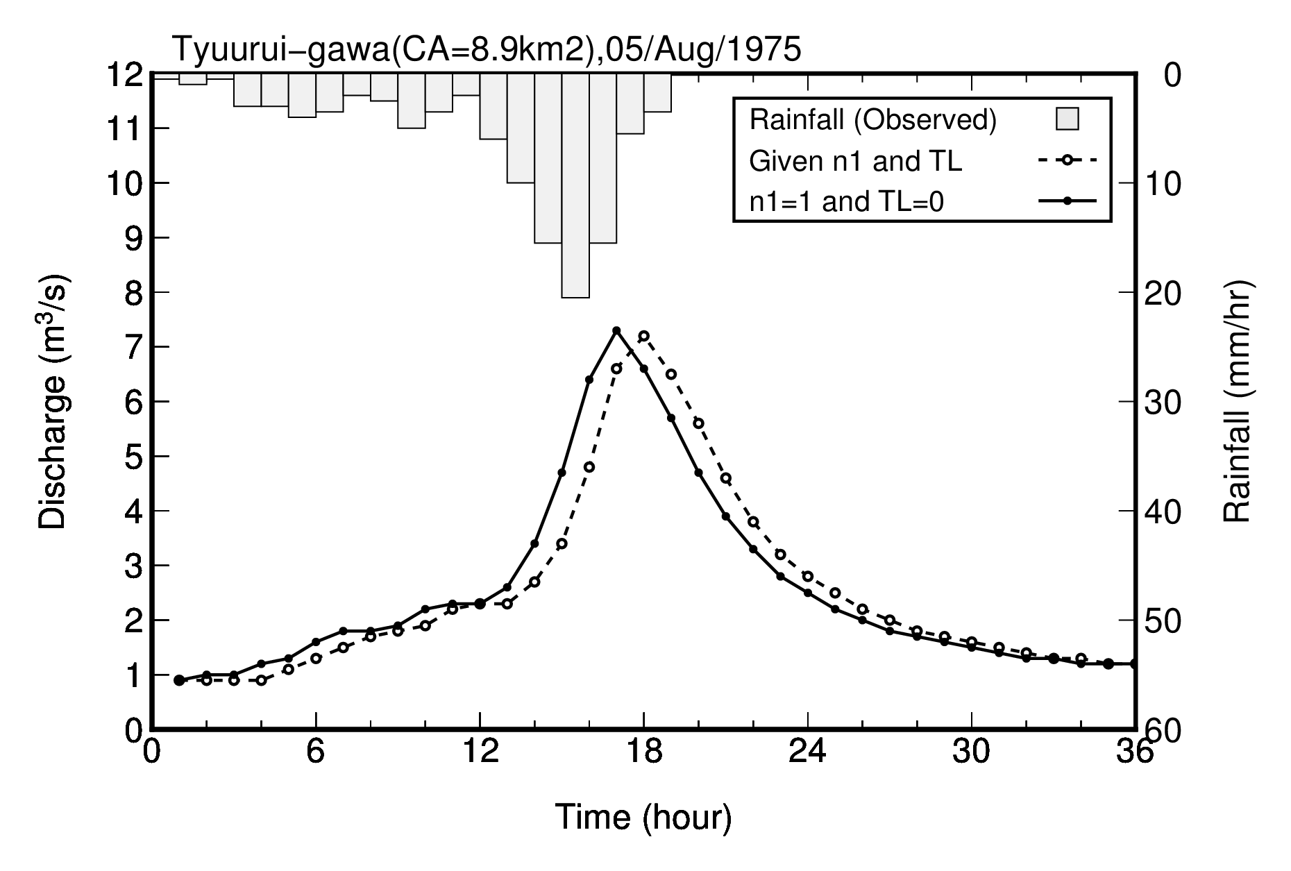
(Source: 椎葉充晴・立川康人・市川温,例題で学ぶ水文学,森北出版株式会社,20120年5月21日in Japanese character) - Case 3 : Tyuuruigawa-river (05/Aug/1975)
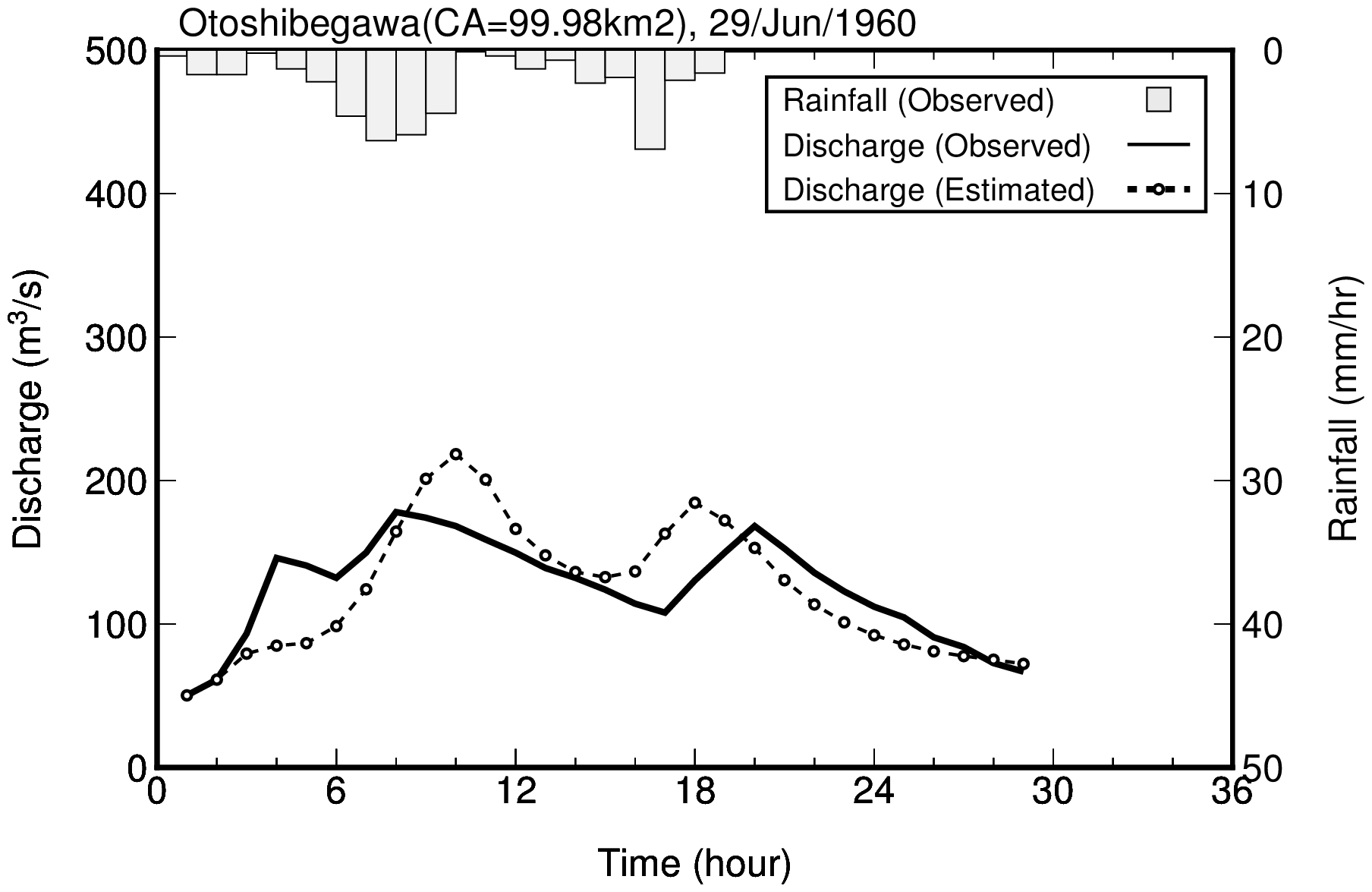
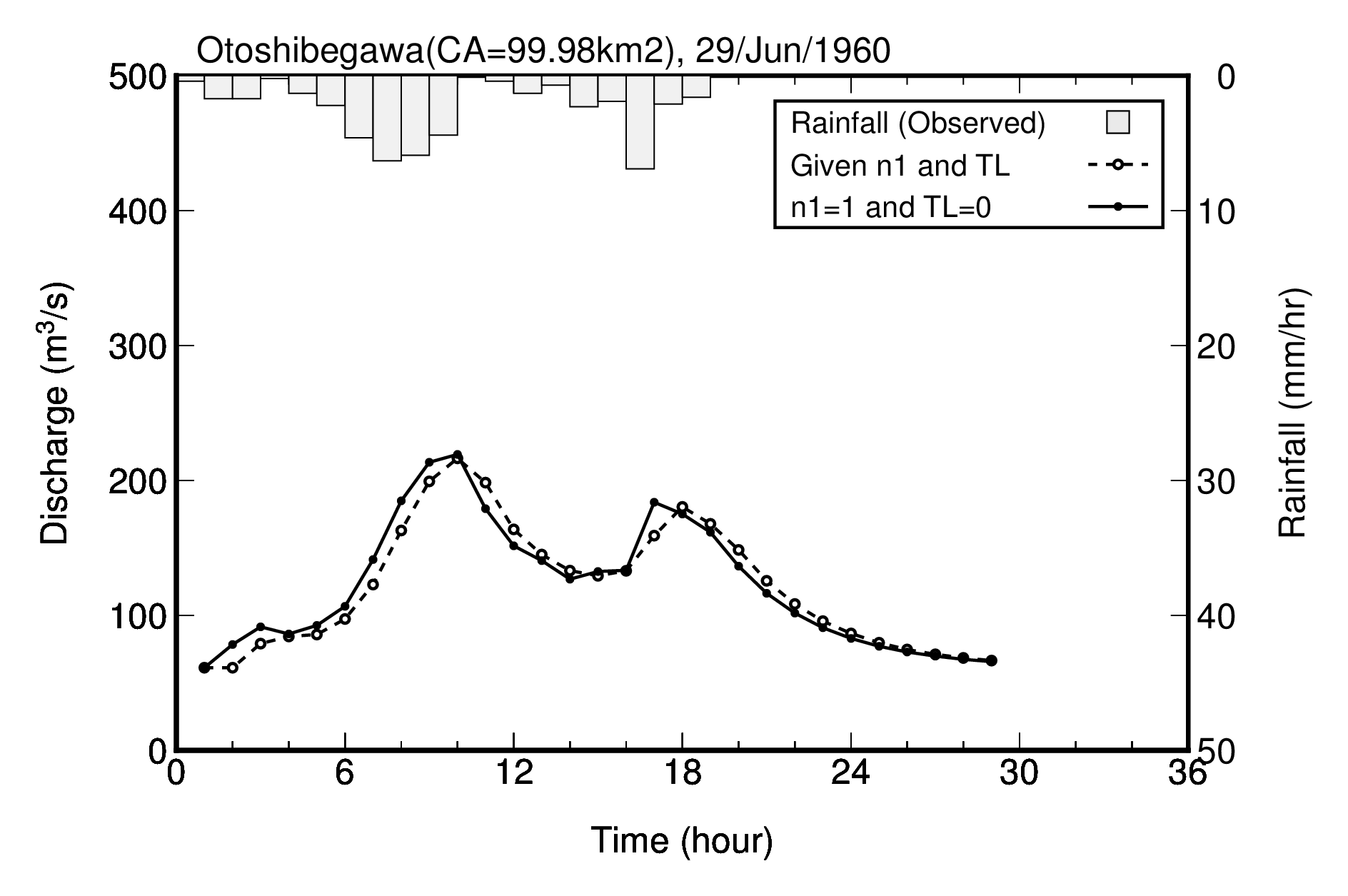
(Source: 北海道開発局土木試験所河川研究室:実用的な洪水流出計算法,昭和62年3月in Japanese character) - Case 4 : Otoshibegawa-river (29/Jun/1960)
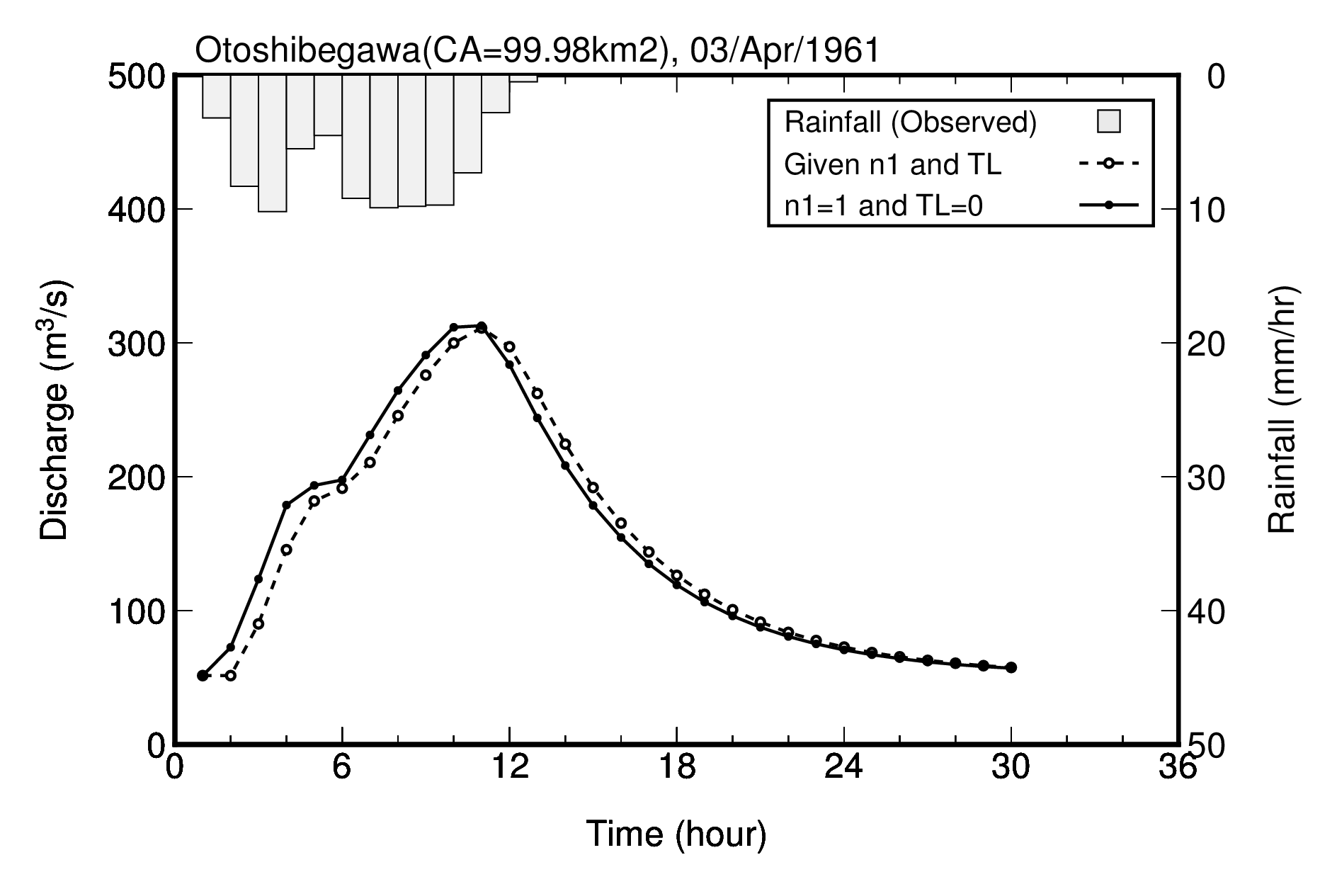
(Source: 実用的な洪水流出計算法 (洪水データ集) in Japanese character) - Case 5 : Otoshibegawa-river (03/Apr/1961)
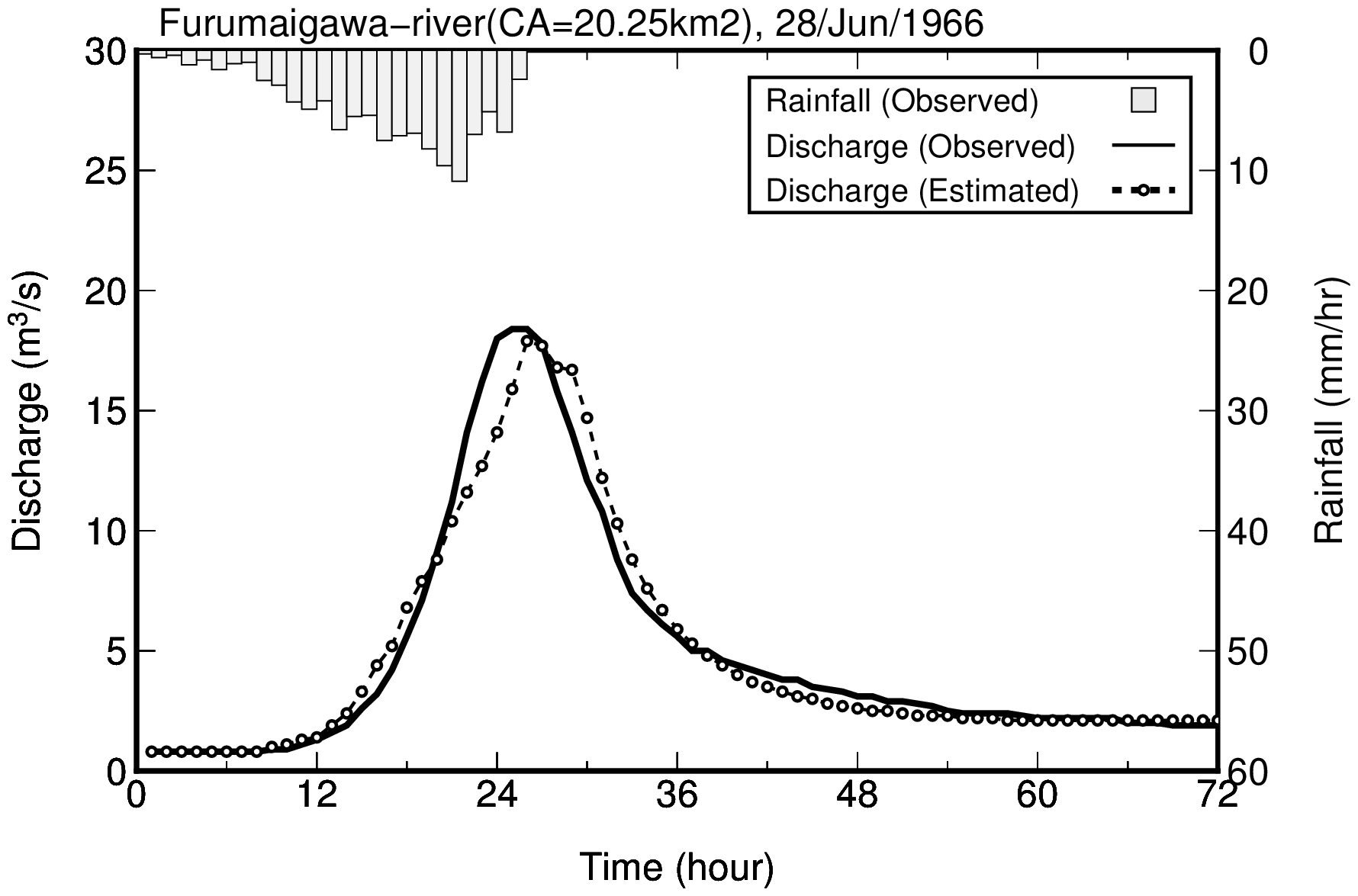
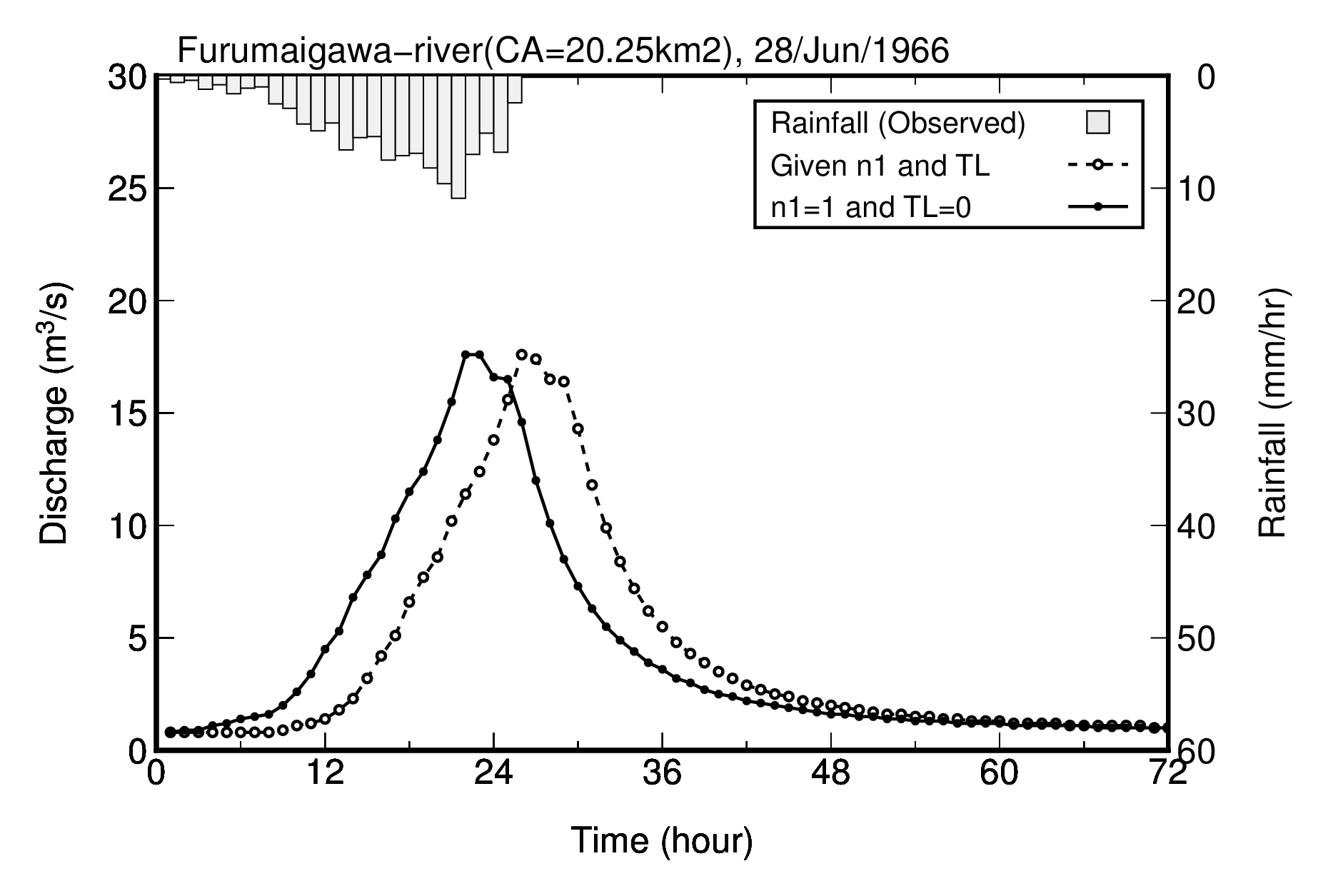
(Source: 実用的な洪水流出計算法 (洪水データ集) in Japanese character) - Case 6 : Furumaigawa-river (28/Jun/1966)
(Source: 実用的な洪水流出計算法 (洪水データ集) in Japanese character)
After this, the relationship between direct run-off and storage, and re-producted Hydrograph using analized parameters are shown for each case.
Case 1: Mukawa-river (09/August/1992)
 |
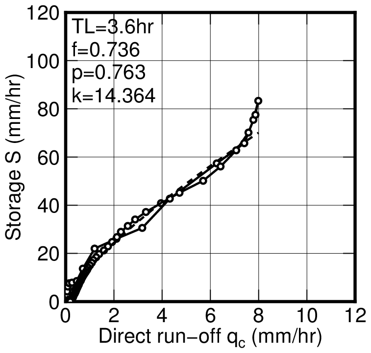 | ||||||||||||||
| TL=0 | TL=3.6hr (adopted) | ||||||||||||||
|---|---|---|---|---|---|---|---|---|---|---|---|---|---|---|---|
| qc-S relationship | |||||||||||||||
 | |||||||||||||||
| Hydrograph for Case 1 | |||||||||||||||
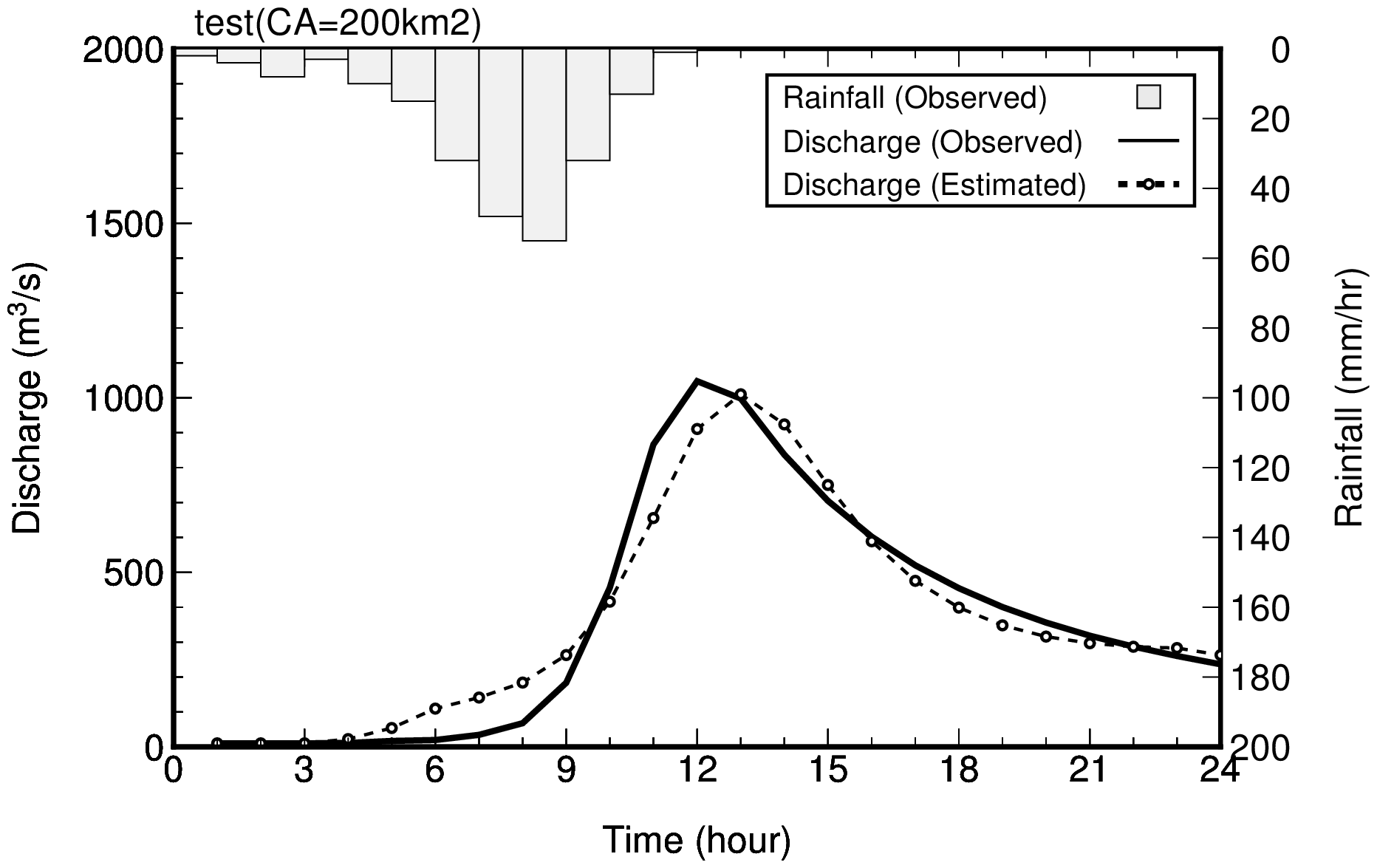
Case 2: Example from textbook
 |
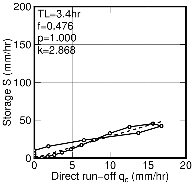 | ||||||||||||||
| TL=0 | TL=3.4hr (adopted) | ||||||||||||||
|---|---|---|---|---|---|---|---|---|---|---|---|---|---|---|---|
| qc-S relationship | |||||||||||||||
 | |||||||||||||||
| Hydrograph for Case 2 | |||||||||||||||
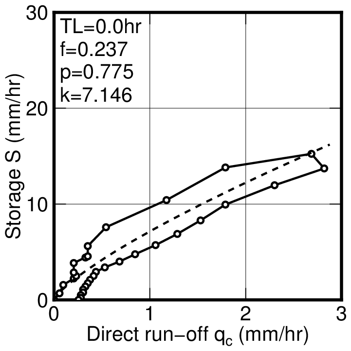
Case 3: Tyuuruigawa-river (05/August/1975)
 |
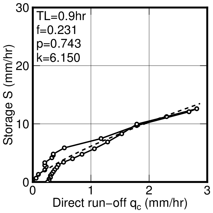 | ||||||||||||||
| TL=0 | TL=0.9hr (adopted) | ||||||||||||||
|---|---|---|---|---|---|---|---|---|---|---|---|---|---|---|---|
| qc-S relationship | |||||||||||||||
 | |||||||||||||||
| Hydrograph for Case 3 | |||||||||||||||
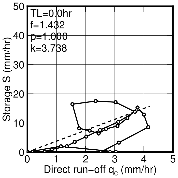
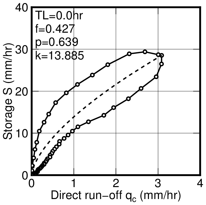
Case 4: Otoshibegawa-river (29/June/1960)
 |
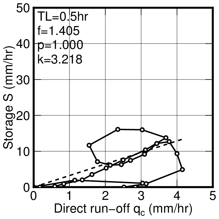 | ||||||||||||||
| TL=0 | TL=0.5hr (adopted) | ||||||||||||||
|---|---|---|---|---|---|---|---|---|---|---|---|---|---|---|---|
| qc-S relationship | |||||||||||||||
 | |||||||||||||||
| Hydrograph for Case 4 | |||||||||||||||
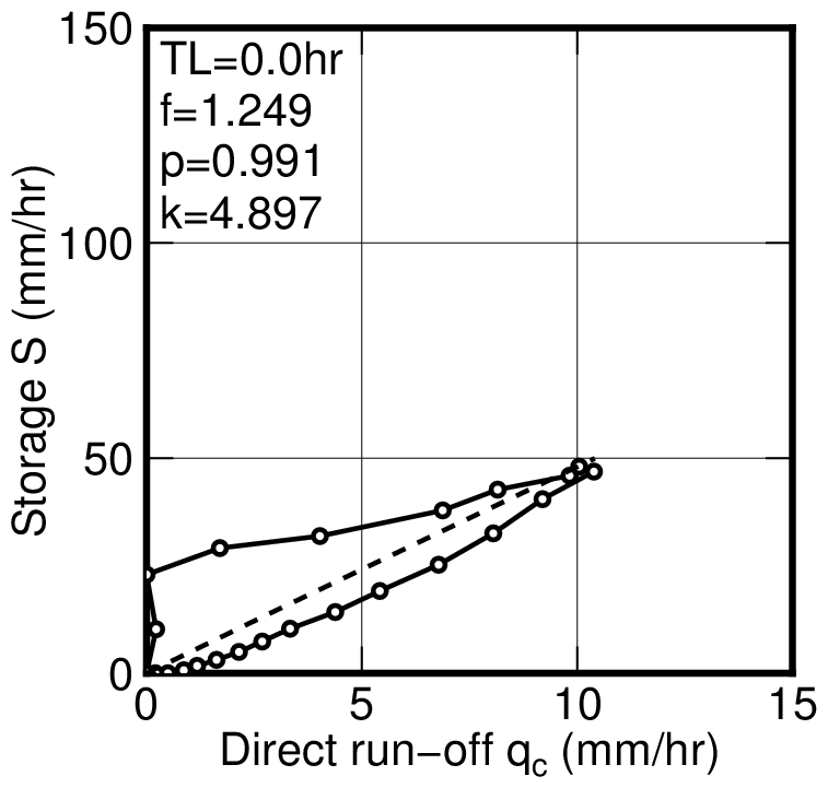
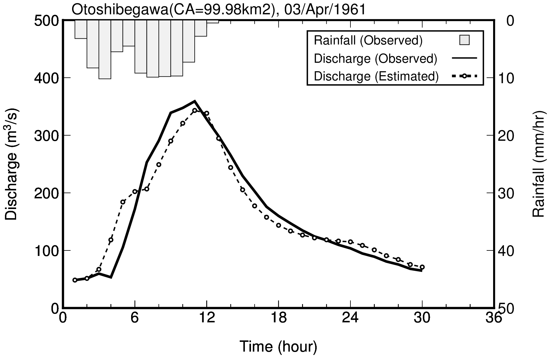
Case 5: Otoshibegawa-river (03/April/1961)
 |
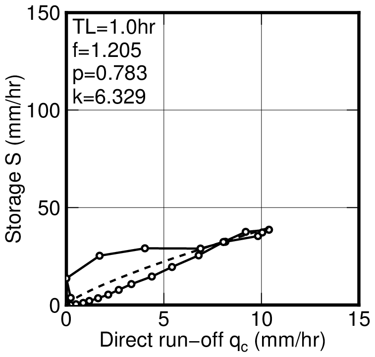 | ||||||||||||||
| TL=0 | TL=1.0hr (adopted) | ||||||||||||||
|---|---|---|---|---|---|---|---|---|---|---|---|---|---|---|---|
| qc-S relationship | |||||||||||||||
 | |||||||||||||||
| Hydrograph for Case 5 | |||||||||||||||
Case 6: Furumaigawa-river (28/June/1966)
 |
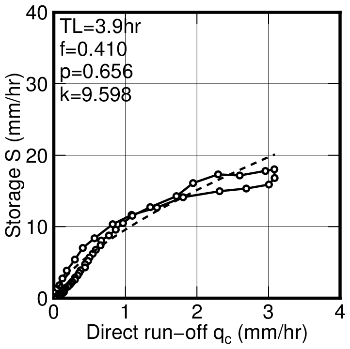 | ||||||||||||||
| TL=0 | TL=3.9hr (adopted) | ||||||||||||||
|---|---|---|---|---|---|---|---|---|---|---|---|---|---|---|---|
| qc-S relationship | |||||||||||||||
 | |||||||||||||||
| Hydrograph for Case 6 | |||||||||||||||
References
- http://www.scj.go.jp/ja/member/iinkai/bunya/doboku/takamizu/pdf/haifusiryou04-1.pdf
(角屋睦,永井昭博:流出解析法 (その10) -- 4.貯留法-貯留関数法による洪水流出解析 --,農業土木学会誌第48巻第10号,pp43-50,1980年10月 in Japanese character) - http://kankyou.ceri.go.jp/genba/suimon.html
(若手水文学研究会:現場のための水文学(1) -- 流出解析 その1 -- in Japanese character) - ISBN 978-4-627-49631-6 published 05.2010 (textbook)
(椎葉充晴・立川康人・市川温,例題で学ぶ水文学,森北出版株式会社,2010年5月21日 in Japanese character) - http://river.ceri.go.jp/contents/tool/kouzui.html
(北海道開発局土木試験所河川研究室:実用的な洪水流出計算法,昭和62年3月 in Japanese character) - http://river.ceri.go.jp/contents/tool/kouzui.html
(実用的な洪水流出計算法 (洪水データ集) in Japanese character)
Program lists
| Filename | Description |
|---|---|
| a_f90.txt | Shell script for execution |
| f90_sfm.f90 | Run-off parameter estimation by Storage Function Method |
| a_gmt_ctl_sfm.txt | GMT command for Hydrograph (control) |
| a_gmt_plt_sfm.txt | GMT command for Hydrigraph (drawing) |
| a_gmt_ctl_qcss.txt | GMT command for qc-S relationship (control) |
| a_gmt_plt_qcss.txt | GMT command for qc-S relationship (drawing) |
| dat_sfm1.csv | Input data sample (1) |
| dat_sfm2.csv | Input data sample (2) |
| dat_sfm3.csv | Input data sample (3) |
| dat_sfm4.csv | Input data sample (4) |
| dat_sfm5.csv | Input data sample (5) |
| dat_sfm6.csv | Input data sample (6) |
Programing
The command for execution of Fortran program is shown below:
./f90_sfm fnameR fnameW n1 m md
| fnameR | Input file name |
| fnameW | Output file name |
| n1 | Starting point of separation of base run-off |
| m | Run-off separation method (0: horizontal separation [constant value], 1: sloped line separation) |
| md | Number of devision of time increment (integer which shall be greater than or equal to one) |
- Start point of direct run-off $n_1$ is inputted as a command line argument.
- About the treatment of the end point of direct run-off $n_2$, is inputted as a command line argument.
- In case of $m=0$, the value of base run-off $q_B$ is constant and the value of it is equal to the value at the start point of direct run-off.
- In case of $m=1$, the value of base run-off $q_B$ is variable from the value at $n_1$ to the value at $n_2$. The end point of direct run-off $n_2$ is estimated automatically.
- The condition of estimation of $n_2$ is the minimum difference between obsedved from and re-producted flow in Hydrograph.
- In practical calculation, $n_2$ is changed from large value to small value.
- Since the value of direct run-off $q_c$ shall be greater than or equal to zero, the values of direct run-off $q_c$ are amended to zero if they are less than zero.
- The estimation method of delay time is shown below.
- Although it is known that the relationship between direct run-off $q_c$ and storage $S$ becomes like a loop shape, the parameters of $p$ and $k$ can be calculated using a regression analysis on log-log graph.
- By shifting the time for effective rainfall, the delay time $T_L$ can be obtained when the residual error between observed data and estimated data by regression analysis becomes minimum value.
- For the regression analysis to calculate the constants $p$ and $k$, special method is adopted to consider the loop shape of $q_c$-$S$ relationship.
The data selection method is shown below:
- Divide the area in horizontal axis $q_c$ to some small areas.
- Chose the maximum and minimum values of $S$ from each area.
- Do the regression analysis using the total datasets which are selected from each small area.
- The upper limit of value of $p$ is set as 1.0. If the value of $p$ exceed 1.0 is obtained by calculation, $p$ is set by 1.0 and $k$ is re-calculated under the condition of $p=1.0$.
- The number of devision of time increment for numerical integration cam be changeable. It is inputted as a number of $md$ of a command line argument. Discharge data is interpolated by Spline interpolation, and rainfall data is set as same value during one hour because the unit of rainfall is 'mm/h'.
- After obtaining the values of $T_L$, $k$ and $p$, Runge-Kutta method is used as a numerical integration method in order to re-product Hydrograph.
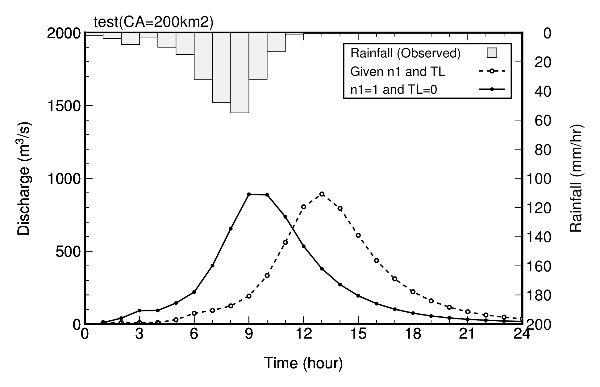
Hydrograph for given parameters
Programs
| Filename | Description |
|---|---|
| a_f90.txt | Shell script for execution |
| f90_sfmq.f90 | Calculation of flood discharge |
| a_gmt_ctl_sfmQ.txt | GMT command for Hydrograph (control) |
| a_gmt_plt_sfmQ.txt | GMT command for Hydrograph (drawing) |
| dat_sfm1Q.csv | Input data sample (1) |
| dat_sfm2Q.csv | Input data sample (2) |
| dat_sfm3Q.csv | Input data sample (3) |
| dat_sfm4Q.csv | Input data sample (4) |
| dat_sfm5Q.csv | Input data sample (5) |
| dat_sfm6Q.csv | Input data sample (6) |
Drawings
 |
 |
 |
| fig_SFM1Q.png | fig_SFM2Q.png | fig_SFM3Q.png |
|---|---|---|
 |
 |
 |
| fig_SFM4Q.png | fig_SFM5Q.png | fig_SFM6Q.png |