Basic formulas for analysis
Displacement at tunnel surface in radial direction
\begin{align}
&\text{Elastic state}&~&u_a = a \cdot \frac{1+\nu}{E} (P_0 - P_i) \\
&\text{Plastic state}& &u_a = \cfrac{R^2}{a} \cdot \cfrac{1+\nu}{E} \cdot \cfrac{\zeta-1}{\zeta+1} \left(P_0 + \cfrac{q_u}{\zeta-1}\right) \qquad
R = a \left(\cfrac{2}{\zeta+1} \cdot \cfrac{P_0 + q_u ~/~ (\zeta-1)}{P_i + q_u ~/~ (\zeta-1)} \right)^{\frac{1}{\zeta-1}}
\end{align}
Condition for plastic zone occurrence
\begin{equation}
P_i \leqq \cfrac{2 P_0 - q_u}{\zeta+1} \qquad \zeta=\cfrac{1+\sin \phi}{1-\sin \phi} \qquad q_u=\cfrac{2 c \cos \phi}{1-\sin \phi}
\end{equation}
| where, | $u_a$ | : Radial displacement at tunnel wall | | $R$ | : Radius of the plastic zone |
| | $a$ | : Radius of tunnel excavation | | $q_u$ | : Uniaxial compressive stress of the ground |
| | $P_0$ | : Ground pressure | | $c$ | : Cohesion |
| | $P_i$ | : Support pressure | | $\phi$ | : Internal friction angle |
| | $E$ | : Elastic modulus of the ground | | $\zeta$ | : Passive earth pressure coefficient |
| | $\nu$ | : Poisson's ratio of the ground | | | |
Support pressure
The support pressure $P_i$ can be obtained using following equation.
\begin{equation}
P_i=P_{sc}+P_{rb}+P_{sr}=\cfrac{\sigma_{sc} t_{sc}}{a}+\cfrac{\sigma_{rb} A_{rb}}{s_t s_l}+\cfrac{\sigma_{sr} A_{sr}}{s_r a}
\end{equation}
| where, | $P_i$ | : Total support pressure |
| | $P_{sc}$ | : Support pressure by Shotcrete |
| | $P_{rb}$ | : Support pressure by Rockbolt |
| | $P_{sr}$ | : Support pressure by Steel Rib |
| | $a$ | : Tunnel excavation radius |
| | $\sigma_{sc}$ | : Stress of Shotcrete |
| | $t_{sc}$ | : Thickness Shotcrete |
| | $\sigma_{rb}$ | : Stress of Rockbolt |
| | $A_{rb}$ | : Section area of Rockbolt |
| | $s_t$ | : Installatio pitch of Rockbolts in circular direction |
| | $s_l$ | : Installation pitch of Rockbolt in tunnel axis direction |
| | $\sigma_{sr}$ | : Stress of Steel Rib |
| | $A_{sr}$ | : Section area of Steel Rib |
| | $s_r$ | : Installation pitch of Steel Rib in tunnel axis direction |
Stress of Shotcrete
The compressive strength of the shotcrete is a function of the age, and the elastic modulus is also a function of the age.
In addition, the stress of the shotcrete may not be equal to its compressive strength.
Therefore, stress increment shall be considered to calculate the shotcrete stresses,
and it can be expressed using the age variable $t$ as follow:
\begin{equation}
\sigma_{sc}(t+\Delta t)=\sigma_{sc}(t)+E_{sc}(t+\Delta t/2) \times \cfrac{\Delta u_a}{a}
\end{equation}
Where, $\Delta u_a$ is the displacement increment in the radial direction during the small time $\Delta t$,
and $\Delta u_a / a$ means the strain increment of the shotcrete in the circumferential direction.
Stress of Rockbolt
The stress of the rockbolt $\sigma_{rb}$ can be obtained using following equation.
\begin{equation}
\sigma_{rb}=E_{rb} \times \cfrac{u_a(t)-u_b(t)}{L}
\end{equation}
Where, $u_a(t)$ is the tunnel surface displacement at shotcrete age $t$ and $u_b(t)$ is the displacement of the end point of the rockbolt at the shotcrete age $t$.
$L$ is the length of the rockbolt, and it can be understood that the second term on right side means the elongation of the rockbolt.
If the value $\sigma_{rb}$ reachs to the yeild strength, it is set to the yeild strength of the rockbolt.
$u_b(t)$ can be calculated as a function of $u_a(t)$ using following equations.
\begin{align}
&\text{Elastic state}&~&u_b(t) = u_a(t) \cfrac{a}{a+L} \\
&\text{Plastic state}& &u_b(t) = \cfrac{R^2}{a+L} \cdot \cfrac{1+\nu}{E} (P_0 - P_R) \\
& & &P_R=\cfrac{2 P_0-q_u}{\zeta+1} \qquad a < R=\sqrt{u_a(t) \cdot a \cdot \cfrac{E}{1+\nu} \cdot \cfrac{\zeta+1}{P_0 (\zeta-1)+q_u}}
\end{align}
Where, $R$ is the boundary between the elastic zone and the plastic zone, and $P_R$ is the support pressure at the boundary $R$.
Stress of Steel Rib
The stress of the steel rib $\sigma_{sr}$ can be obtained using following equation.
\begin{equation}
\sigma_{sr}=E_{sr} \times \cfrac{u_a(t)-u_a(0)}{a}
\end{equation}
Where, $u_a(t)$ is the tunnel surface displacement at shotcrete age $t$ and $u_a(0)$ is the tunnel surface displacement at the shotcrete age 0.
It can be understood that the second term on right side means the strain in the circumferential direction.
If the value $\sigma_{sr}$ reachs to the yeild strength, it is set to the yeild strength of the steel rib.
Critical strain
The critical strain which was advanced by Dr.Sakurai is often used for the calculation of the trigger level displacement for NATM.
And it is thought that the possibility of abnormal observation is very low,
if the circumferential strain of tunnel surface is less than the critical strain of the ground material.
The critical strain $\epsilon_0$ and the wall displacement $u_{a0}$ corresponding to the critical strain can be expressed as follow.
\begin{equation}
u_{a0}=a \times \epsilon_0 \times 0.01 \qquad \epsilon_0= \alpha \times (UCS \times 10)^{-0.3}
\end{equation}
| where, | $u_{a0}$ | : Radial displacement of the tunnel wall corresponding to a critical strain |
| | $UCS$ | : Uniaxial compressive strength of an intact rock (unit: MPa) |
| | $\epsilon_0$ | : Critical strain of the ground material (unit: %) |
| | $\alpha$ | : Coefficient Critical strain of the ground material (unit: %) |
(Note)
$\alpha$ is approximately equal to 2.4 for the intermediate value of the critical strain by Dr.Sakurai
which is shown in the paper 'An Evaluation Technique of Displacement Measurements
in Tunnels' by Dr.Sakurai (1982).
It should be noted that the unit of the calculated critical strain $\epsilon_0$ is '%', and
$UCS$ is quite different from $q_u$ which is an uniaxial compressive strength of a rock mass.
|
Estimation of cohesion of bedrock
If a pseudo-yeild strain $\epsilon_y$ is defined, the cohesion of the bedrock $c$ can be estimated using following equations
with given characteristics of $E$, $\nu$ and $\phi$.
\begin{equation}
c=\cfrac{q_u (1-\sin \phi)}{2 \cos \phi} \qquad \text{where,} \quad q_u=\cfrac{2 E}{1+\nu} \cdot \epsilon_y
\end{equation}
One idea to calculate the pseudo-yeild strain $\epsilon_y$ is to use the Elastic modulus and the compressive strength by the uniaxial compressive test.
However, the value $\epsilon_y$ should be larger than the critical strain $\epsilon_0$, and it should be smaller than the strain corresponding to the maximum compressive strength of the rock material.
Special consideration for Plastic state
Generally, Ground Response Curve is drawn using the same strehgth parameter, this means the values of $c$ and $\phi$ are constant in the same analysis case.
However, when the ground pressure release rate depending on the excavation progress will be considered using the same strehgth parameters,
the plastic zone under the lower support pressure sometimes returns to the elastic zone under the higher support pressure.
If we don't want to see this phenomenon, it is one idea that the displacement at start point of plastic zone occurance is set to constant value.
In this case, the updated value of $q'_u$ can be expressed as follow, using the assumptions that $\phi$ is constant and $c$ will be changed depending on the required support pressure $P$.
\begin{equation}
q'_u=2 P - P_{cr} \cdot (1+\zeta) \qquad P_{cr}=P - q_u / 2
\end{equation}
| where, | $q'_u$ | : Updated uniaxial compressive strength of the ground
This value is changed for each pressure release rate. |
| | $P$ | : Required support pressure at zero displacement |
| | $P_{cr}$ | : Required support pressure at start point of the plastic zone occurance |
| | $q_u$ | : Initial uniaxial compressive strength of the ground.
This value calculated by initial input $c$ and $\phi$ is constant. |
In above equation, if $q'_u$ becomes less than or equal to zero, $q'_u$ will be set to zero.
Sample calculations and drawings
Equivalent excavation radius for simplified circular cross section
In general, the cross section of a tunnel is not true circle except a tunnel by TBM.
Therefore, to adopt a simplified NATM excavation analysis with circular cross section, it is necessary to assume the equivalent radius of a circle.
As methods to estimate the equivalent radius, followings have been adopted through the many experiances of NATM tunnel excavation.
- One half of the average value of the excavation width and excavation height
- Radius of a circle with the same section area as the original shape
The reason to adopt above method has been thought that above methods gives safety side displacement conveniently in the trigger level study of NATM excavation.
(The smaller radius gives safety side solution in the trigger level study because estimated displacement becomes smaller.)
In this study, it is tried to estimate an equivalent excavation radius using a model dimensions of Type E by 2D-FEM in order to obtain the reasonable equivalent excavation radius.
| Tunnel dimension |
|---|
| Type | Width (mm) | Height (mm) | Average (mm) |
|---|
| Inner size | RC thick. | Shotcrete | Outer size |
Inner size | RC thick. | Shotcrete | Outer size |
|---|
| A | 5000 | 400 x 2 | --- | 5800 | 4600 | 400 x 2 | --- | 5400 | 5600 |
| B | 5000 | 400 x 2 | 50 x 2 | 5900 | 4600 | 400 x 2 | 50 | 5450 | 5675 |
| C | 5000 | 400 x 2 | 100 x 2 | 5900 | 4600 | 400 x 2 | 50 | 5450 | 5675 |
| D | 5000 | 400 x 2 | 150 x 2 | 6000 | 4600 | 400 x 2 | 100 | 5500 | 5750 |
| E | 5000 | 400 x 2 | 200 x 2 | 6000 | 4600 | 400 x 2 | 100 | 5500 | 5750 |
The model tunnel has 6.0m width and 5.5m height, and used FEM model and the displacement mode are shown below.
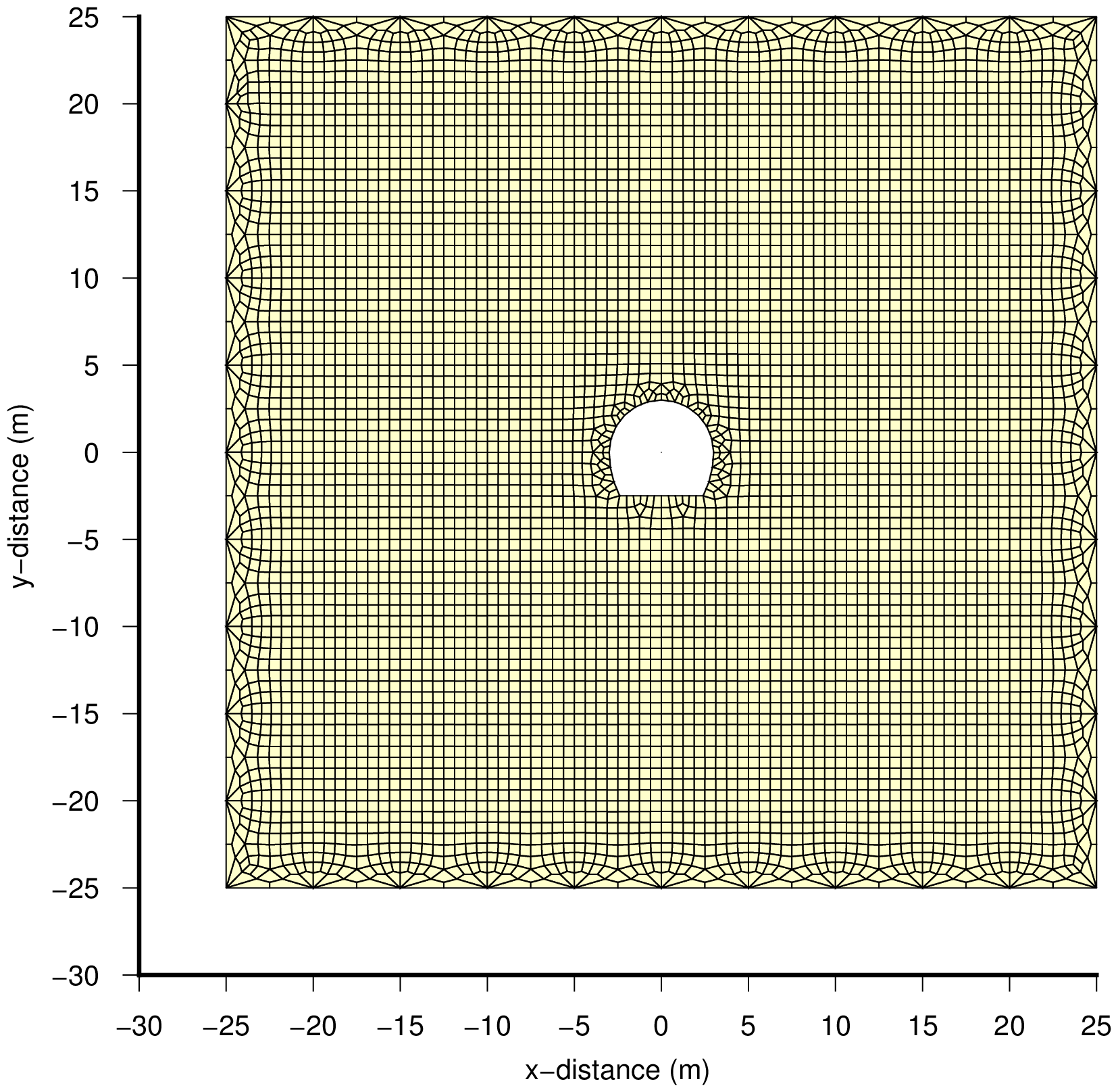 |
(1)Analysis model
Plane strain, elastic state
(2)Tunnel shape
Width=6.0m, Height=5.5m
Upper arc radius=3.0m
Lower arc radius=5.5m
(3)Analysis steps
a. Fix the outside nodes and tunnel surface nodes
b. Give the initial stresses to all elements
(vertical: 2.0MPa)
(horizontal: 2.0MPa)
c. Calculate the nodal forces of the tunnel surface nodes
d. Load the nodal forces to the tunnel surface nodes
in the opposite direction.
d. Calculate the nodal displacements
|
| Analysis model |
|---|
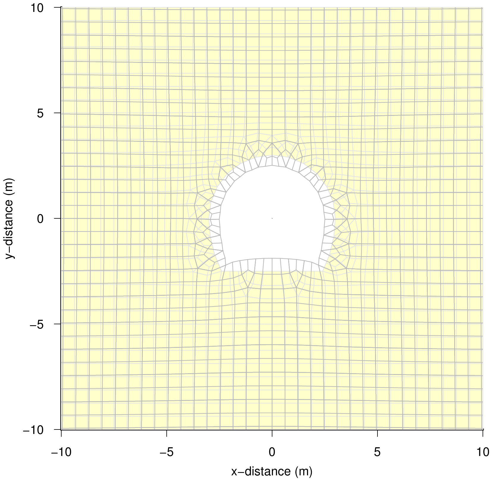 |
| Displacement mode |
|---|
The results of comparison of the tunnel surface displacements are shown below.
| FEM model | $P_0$
(MPa) | $E$
(MPa) | $\nu$ | Disp.by FEM (mm) | Equivalent radius
as a citcle (mm) |
|---|
| Croun | SL | Invert |
|---|
Width=6.0m
Height=5.5m
Constant section
|
2.0 | 2000 | 0.25 | 3.641 | 3.742 | 4.755 | 2994 |
| 2.0 | 1000 | 0.25 | 7.282 | 7.485 | 9.509 | 2994 |
| 2.0 | 500 | 0.25 | 14.563 | 14.969 | 19.019 | 2994 |
| 2.0 | 300 | 0.30 | 25.093 | 25.695 | 31.906 | 2965 |
| 2.0 | 100 | 0.30 | 75.278 | 77.086 | 95.718 | 2965 |
| Equation for Equivalent radius calculation: $a=\frac{E}{1+\nu} \frac{u}{P_0}$ |
| ($a$: radius, $u$: displacement) |
| As a displacement 'u', the value of the spring line (SL) was used. |
Comments for above results are shown below.
- It is understandable that the estimated equivalent radius is almost the same as a half of the FEM model width of W=3.0m.
- The difference of the equivalent radius between the set of A,B,C and the set of D,E is caused by the difference of Poisson's ratio.
- The displacement at the invert is the largest value in comparison with the displacement at the crown and spring line.
This can be always observed in the numerical analysis by FEM.
However, it is not necessary to focus to the invert displacement except special condition such as an expansible ground,
because the invert is filled by excavated muck and compacted by excavators and dump trucks every day.
Therefore, the displacement of SL which is larger than that of Crown can be used for the calculation of the equivalent radius.
As a result, the equivalent radiuses can be obtained as follows using the result of 2D FEM.
| Setting of equivalent radius |
|---|
| Type | Inner size
(mm) | RC thick.
(mm) | Shotcrete
(mm) | Outer size
(mm) | Equivalent radius
(mm) |
|---|
| A | 5000 | 400 x 2 | --- | 5800 | 2894 |
| B | 5000 | 400 x 2 | 50 x 2 | 5900 | 2944 |
| C | 5000 | 400 x 2 | 100 x 2 | 5900 | 2944 |
| D | 5000 | 400 x 2 | 150 x 2 | 6000 | 2965 |
| E | 5000 | 400 x 2 | 200 x 2 | 6000 | 2965 |
| Equivalent radiuses for type D and E are the same as the results by 2D FEM |
| Equivalent radiuses for type A, B, and C |
| (Equivalent radius) = (Outer size) / 2 x 2994 / 3000 |
| All dimensions are widths on the spring line (SL) |
Ground pressure release rate
In the tunnel excavation, followings have been known generally:
- The displacement of the measurement point has been started before cut surface reaching there.
This means that when cut surface reaches the measurement point, some parts of the ground pressure have been released.
- When the distance between cut surface and measurement point reaches to the approximately 3.5 times distance of the excavation diameter, the inner space displacement converges to a constant value.
Considering above, the estimation of the ground pressure release rate was tried using an axisymmetrical FEM model.
The outline of the analysis and results are shown below.
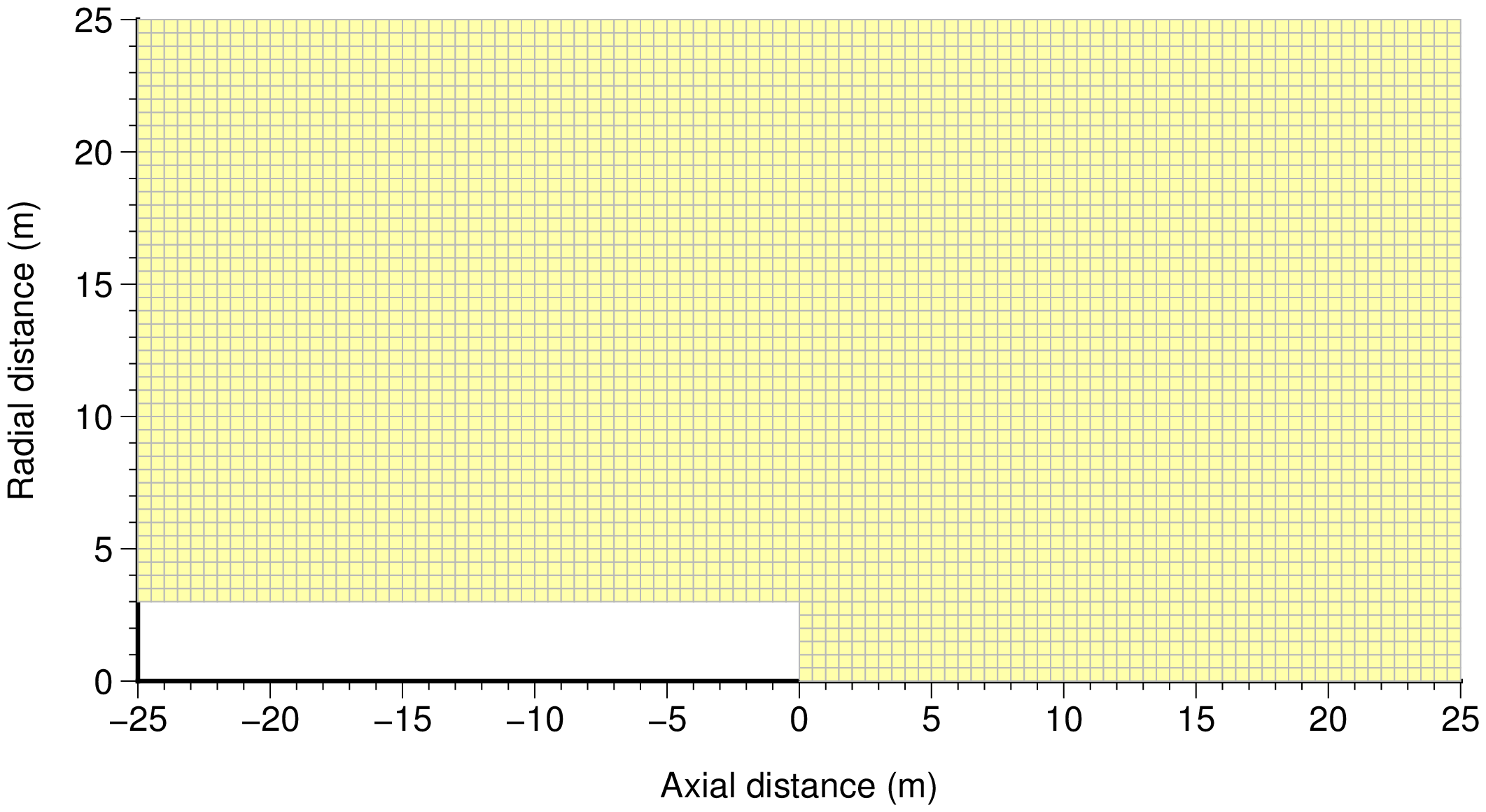 |
(1)Analysis model
Axisymmetrical, elastic state
(2)Tunnel diameter
6m (circular cross section)
(2)Boundary conditions
(sides at x=-25m and x=25m)
Free in radial direction
fixed in axial direction
(3)Loads
2.0MPa at the side r=25m
(compression in radial direction)
|
| Analysis model |
|---|
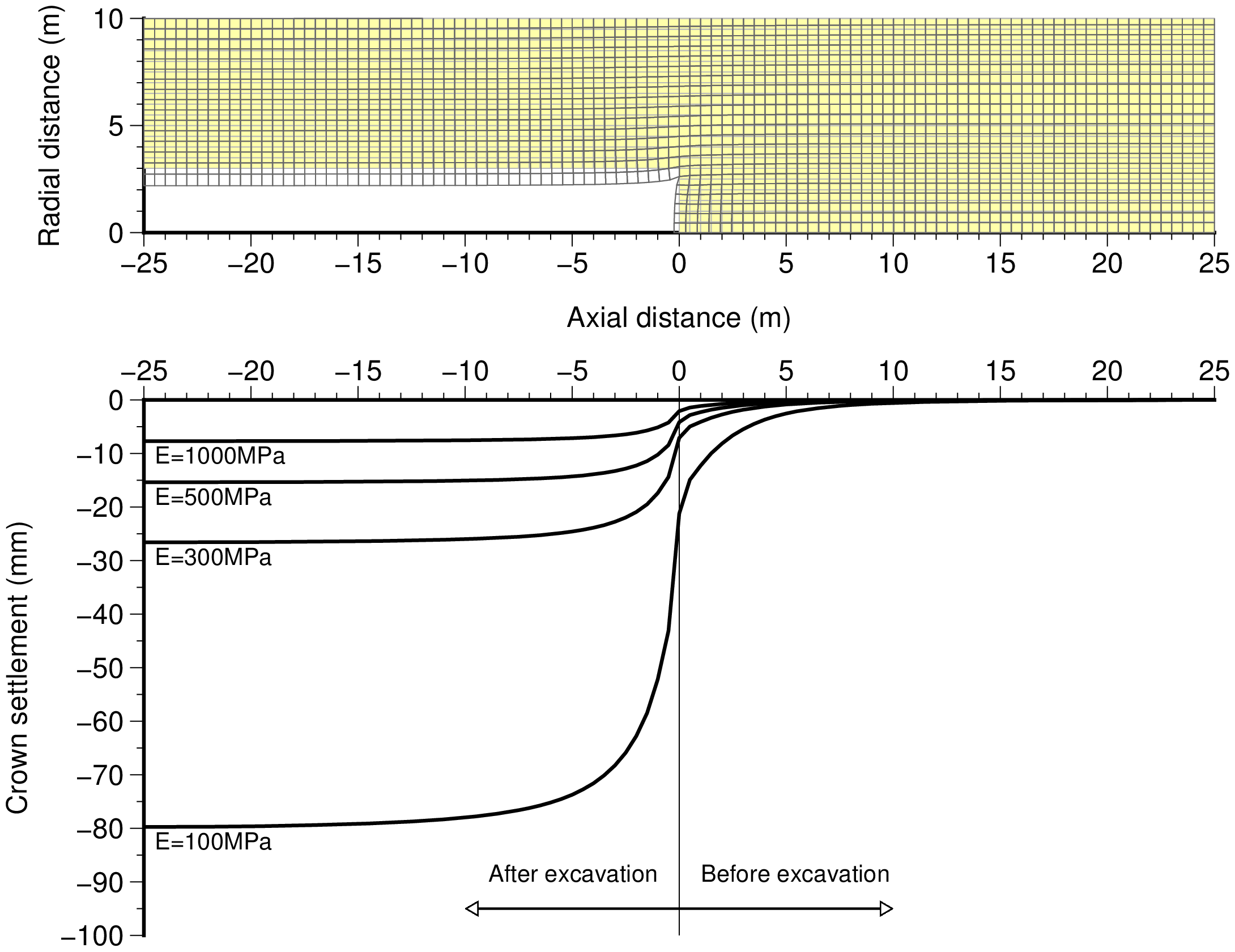 |
| Displacement mode and Crown settlement |
|---|
$E$
(MPa) | $\nu$ | Crown settlement |
|---|
-25.0m
(-4.17D) | -18.0m
(-3.00D) | -6.0m
(-1.00D) | -3.0m
(-0.50D) | -0.5m
(-0.08D) | 0.0m
(0.00D) |
|---|
| 1000 | 0.25 | -7.686
(1.000) | -7.662
(0.997) | -7.273
(0.946) | -6.636
(0.863) | -4.217
(0.549) | -2.074
(0.270) |
| 500 | 0.25 | -15.372
(1.000) | -15.324
(0.997) | -14.546
(0.946) | -13.273
(0.863) | -8.434
(0.549) | -4.148
(0.270) |
| 300 | 0.30 | -26.581
(1.000) | -26.495
(0.997) | -25.059
(0.943) | -22.753
(0.856) | -14.375
(0.541) | -7.069
(0.266) |
| 100 | 0.30 | -79.742
(1.000) | -79.484
(0.997) | -75.176
(0.943) | -68.259
(0.856) | -43.124
(0.541) | -21.208
(0.266) |
| 'D' means the excavation diameter of the tunnel. |
| The values in ( ) mean the dispracement rates to maximum displacement at the distance -25m. |
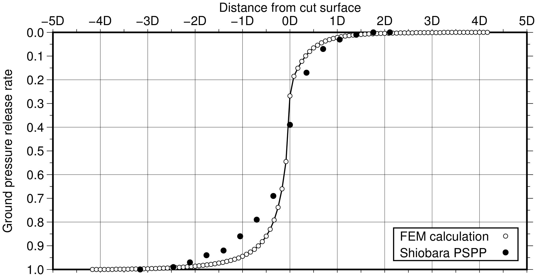
From above, following diagram which is 'relationship between the distance from cut surface and ground pressure release rate' can be obtained, because the ground pressure is proportional to the displacement in the elastic body.
And a measured sample by extensometers at Access tunnel of Shiobara PSPP is shown in the diagram as a reference.
 |
| Ground stress release rate |
|---|
| 'Shiobara': measured example by extensometers at Access tunnel of Shiobara PSPP. |
| 'D' means the excavation diameter of the tunnel. |
| (FEM calculation: D=6.0m, circular cross section) |
| (Shiobara PSPP Access tunnel: D=7.12m, W7.12m x H6.16m) |
In this analysis, following relationship was used based on FEM analysis.
Relationship between the distance from cut surface
and ground pressure release rate |
|---|
| Dist. | 0.00D | 0.25D | 0.50D | 0.75D | 1.00D | 1.25D | 1.50D | 2.00D | 2.50D | 3.00D | 3.50D |
|---|
| GPRR | 0.500 | 0.738 | 0.860 | 0.915 | 0.945 | 0.962 | 0.973 | 0.986 | 0.993 | 0.997 | 1.000 |
|---|
| Dist. : Distance from cut syrface (D: excavation diameter) |
| GPRR : Ground pressure release rate |
At the point 0D (just cut surface), the ground pressure release rate by FEM is less than 0.3.
However, the initial ground pressure release rate for the design has been set to 0.5 generally, because installation space for the support and measuring point shall be considered.
So, the ground pressure rerease rate as an initial value is set to 0.5 in this study.
Conditios for calculations
| Typical support type |
|---|
| Type | Shotcrete | Rockbolt | Steel Rib |
|---|
| A | -- | -- | -- |
| B | SFR40-50mm | -- | -- |
| C | SFR40-50mm | D25 / (2.0m x 2.0m) L=2.0m | -- |
| D | SFR40-100mm | D25 / (1.5m x 1.5m) L=2.0m | -- |
| E | SFR40-100mm | D25 / (1.0m x 1.0m) L=3.0m | H100(A=1920mm$^2$) ctc 1.0m |
| Characteristics of Support members |
|---|
| Member | Characteristics |
|---|
| Shotcrete | Compressive strength | (MPa) | $\sigma_c=7.56 \sqrt{d}$ (d : age in day) |
| Elastic modulus | (MPa) | $E_c=1826 \sqrt{\sigma_c}$ |
| Rockbolt | Yeild strength | (MPa) | $\sigma_{yrb}=226$ |
| Elastic modulus | (MPa) | $E_{rb}=200,000$ |
| Size | | D25 (diameter: 25mm) |
| Steel Rib | Yeild strength | (MPa) | $\sigma_{ysr}=275$ |
| Elastic modulus | (MPa) | $E_{sr}=200,000$ |
| Size | | H-100 (section area=1920 mm$^2$) |
| $E_c$ is set based on the design value of Access tunnel of Shipbara PSPP.
|
| Ground characteristics |
|---|
| Type | $a$
(mm) | $P_0$
(MPa) | $E$
(MPa) | $\nu$ | $c$
(MPa) | $\phi$
(degree) | $UCS$
(MPA) | $\epsilon_0$
(%) | $u_{a0}$
(mm) |
|---|
| A | 2894 | 2.12 | 5000 | 0.25 | 4.21 | 50 | 50 | 0.129 | 3.7 |
| B | 2944 | 2.12 | 3000 | 0.25 | 3.35 | 45 | 30 | 0.150 | 4.4 |
| C | 2944 | 2.12 | 1000 | 0.25 | 1.75 | 40 | 10 | 0.208 | 6.1 |
| D | 2965 | 2.12 | 500 | 0.30 | 1.16 | 35 | 5 | 0.257 | 7.6 |
| E | 2965 | 2.12 | 100 | 0.30 | 0.42 | 30 | 1 | 0.416 | 12.3 |
| Calculation formula for $\epsilon_0$: $\epsilon_0=0.83 \cdot (10 \cdot UCS)^{-0.3}$ |
| Calculation formula for $q_u$: $q_u=2 E / (1+\nu) \cdot 2.25 \epsilon_0$ |
Although the equivalent radius shall be defined as a mechanical character for the NATM excavation analysis,
the excavation daiameter shall be defined as a geometric character for the study of the progress.
Therefore, the average of the tunnel width and height is used as the characteristic of the excavation diameter in below table.
| Daily progress and Required time for displacement convergence |
|---|
| Type | Dia. | Daily progress | Required time for convergence |
|---|
| A | 5.6 m | 9.0 m/day | 2.2 days (5.6m x 3.5 / 9.0m) |
| B | 5.7 m | 7.5 m/day | 2.7 days (5.7m x 3.5 / 7.5m) |
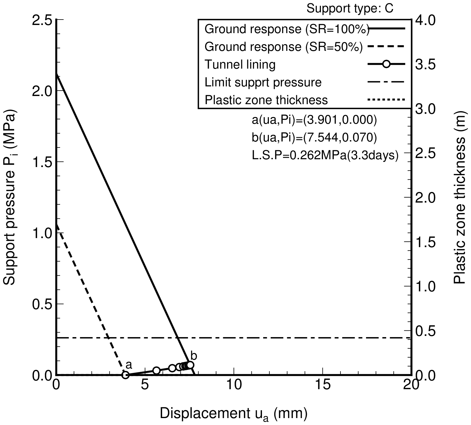
| C | 5.7 m | 6.0 m/day | 3.3 days (5.7m x 3.5 / 6.0m) |
| D | 5.8 m | 4.5 m/day | 4.5 days (5.8m x 3.5 / 4.5m) |
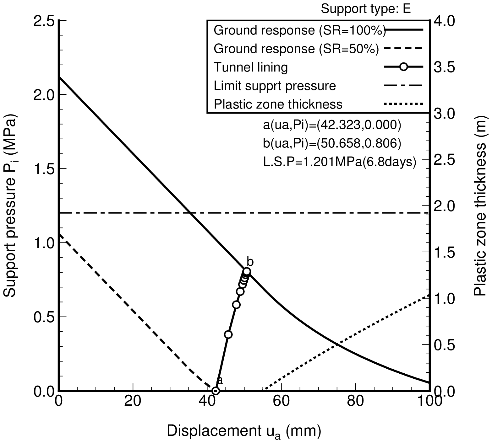
| E | 5.8 m | 3.0 m/day | 6.8 days (5.8m x 3.5 / 3.0m) |
| 'Required time for convergence' is calculated as a time for 3 times diameter progress.
|
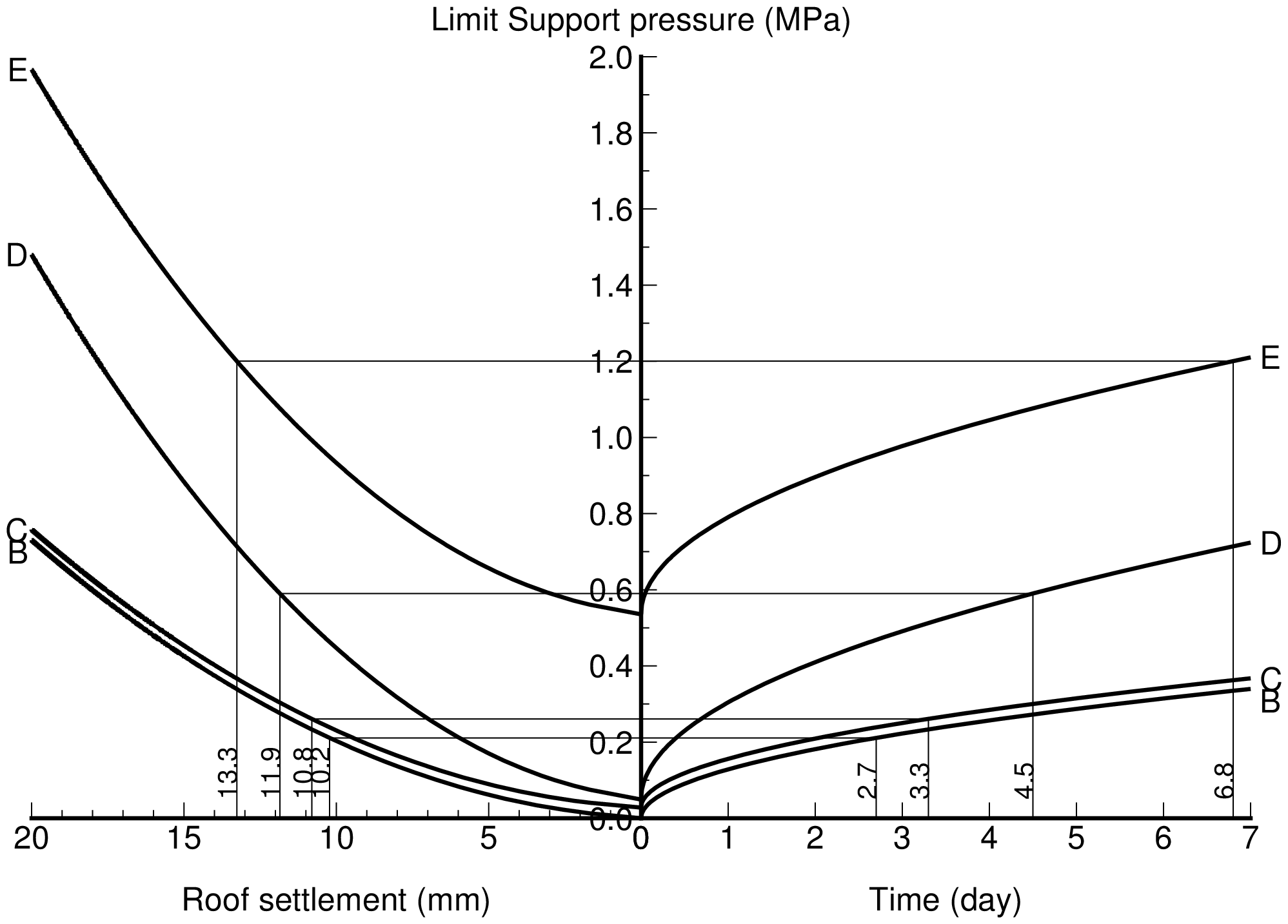
Relationship among Limit support pressure, displacement and age of the support
Limit support presure shown below can be calculated using following assumptions.
- The rockbolts and steel rib display the maximum strengthes of them at time zero and zero displacement.
- The shotcrete stress is always reached to its compressive strength for all calculation time steps.
- The capacity of the displacement increment can be calculated using following equation. This is based on above assumption.
\begin{equation}
\Delta u=a \cdot \Delta \epsilon_c = a \cdot \cfrac{\sigma_c (t+\Delta t)-\sigma_c (t)}{E_c (t+\Delta t/2)}
\end{equation}
| where, | $\Delta u$ | : Displacement increment in radial direction |
| | $a$ | : Excavation radius |
| | $\Delta \epsilon_c$ | : Strain increment of the shotcrete |
| | $\sigma_c$ | : Compressive strength of the shotcrete |
| | $E_c$ | : Elastic modulus of the shotcrete |
| | $t, \Delta t$ | : Time and time increment |
 |
| fig_s.png |
|---|
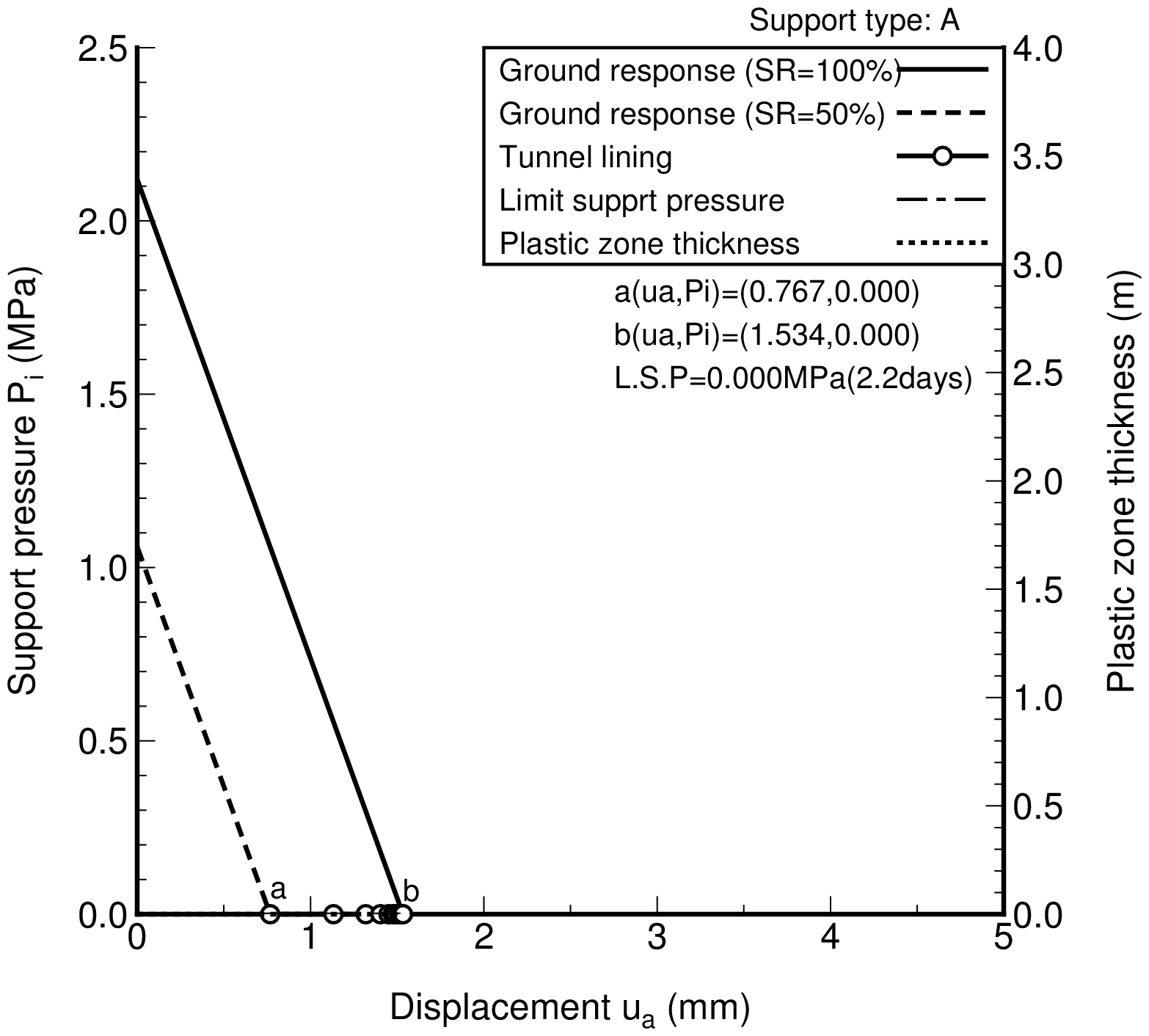
Ground Response Curves and Estimation of Inner space displacements
The displacement and support pressure for each time step can be calculated using the relationship between the displacement and the limit support pressure shown above.
Since this method uses a average rigidity of the support members, the calculated values are only approximate values.
However, it is easy to understand the calculation processes.
From below diagrams, it can be understood that the support systems have adequate strengthes against the expected ground pressure.
 |
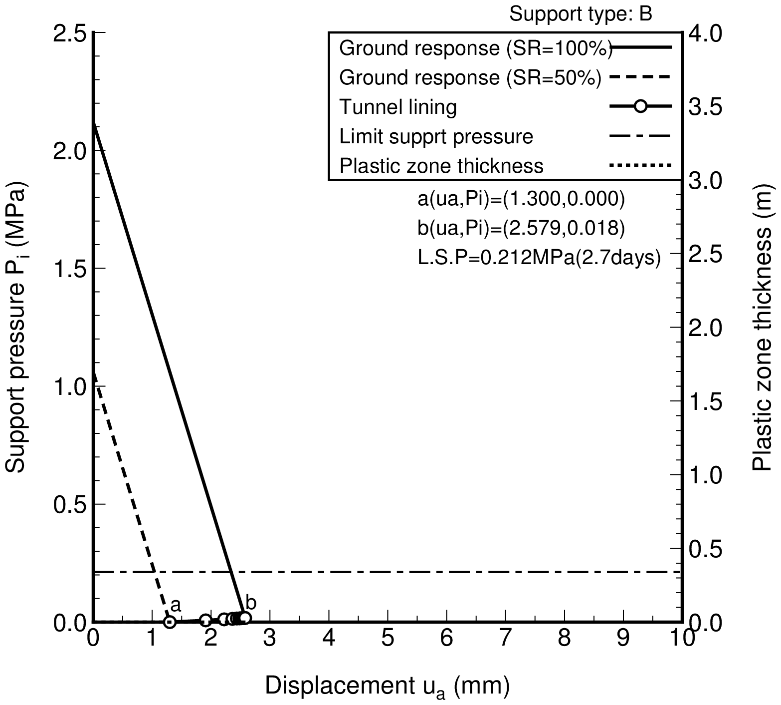 |
| fig_A.png | fig_B.png |
|---|
 |
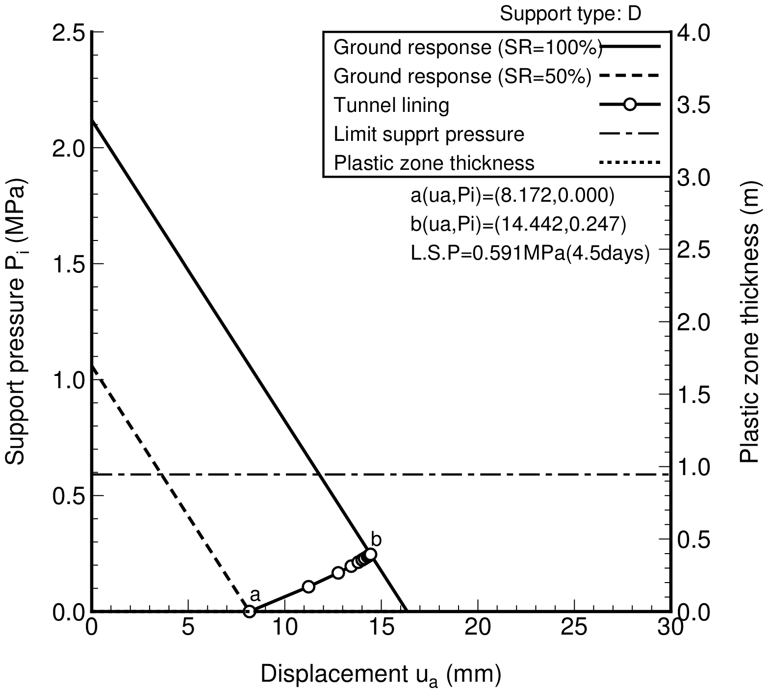 |
| fig_C.png | fig_D.png |
|---|
 |
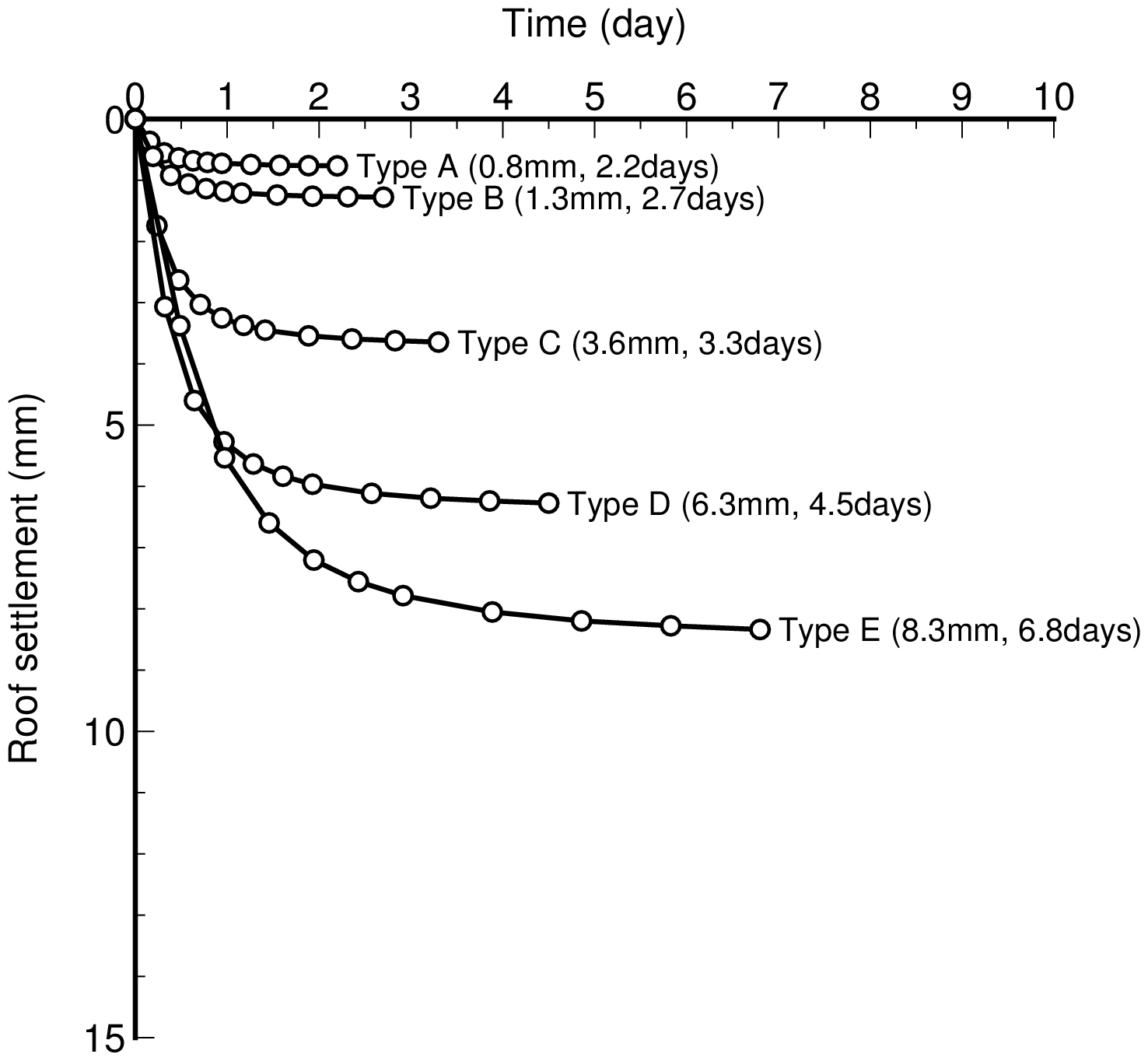 |
| fig_E.png | fig_u.png |
|---|
Summary of displacement calculation
| Type | Day | Total disp. (mm) | Measurable disp. (mm) |
|---|
| $u_{ai}$ | $u_{ae}$ | $u_{a0}$ | $u_{as}$ | $\delta u_{ae}$ | $\delta u_{a0}$ | $\delta u_{as}$ |
|---|
| A | 2.2 | 0.7 | 1.5 | 3.7 | -- | 0.8 | 3.0 | -- |
| B | 2.7 | 1.3 | 2.6 | 4.4 | 11.5 | 1.3 | 3.1 | 10.2 |
| C | 3.3 | 3.9 | 7.5 | 6.1 | 14.7 | 3.6 | 2.2 | 10.8 |
| D | 4.5 | 8.1 | 14.4 | 7.6 | 20.0 | 6.3 | (-0.5) | 11.9 |
| E | 6.8 | 42.3 | 50.6 | 12.3 | 55.6 | 8.3 | (-30.0) | 13.3 |
| where, | Day | : Required time for displacement convergence (corresponding to 3 times diameter progress) |
| | $u_{ai}$ | : Initial displacement at the ground pressure release rate 50% |
| | $u_{ae}$ | : Estimated total displacement with support effect |
| | $u_{a0}$ | : Equivalent displacement to the critical strain of the bedrock |
| | $u_{as}$ | : Equivalent displacement to the support strength at 3 times diameter progress |
| | $\delta u_{ae}$ | : $=u_{ae}-u_{ai}$, measurable displacement considering the support effect |
| | $\delta u_{a0}$ | : $=u_{a0}-u_{ai}$, measurable displacement considering the critical strain |
| | $\delta u_{as}$ | : $=u_{as}-u_{ai}$, measurable displacement considering the support strength |