Contents
In the case of obtaining the design flood discharge or design probable rainfall, it is necessary to calculate the hydrologic statistics.
In this document, formulas and calculation method of the hydrologic statistics are introduced.
Please note that the theorotical details are not mentioned in this document.
Basic issues
PDF and CDF
The relationship between PDF and CDF is shown below:
\begin{equation}
F(x)=\int_{-\infty}^x f(t) dt
\end{equation}
| where, | $f(x)$ | : PDF (probability density function) |
| | $F(x)$ | : CDF (cumulative distribution function |
According to the definition of CDF, we can understand that $F(x)$ : CDF is equal to non-exceedance probability for $x$ .
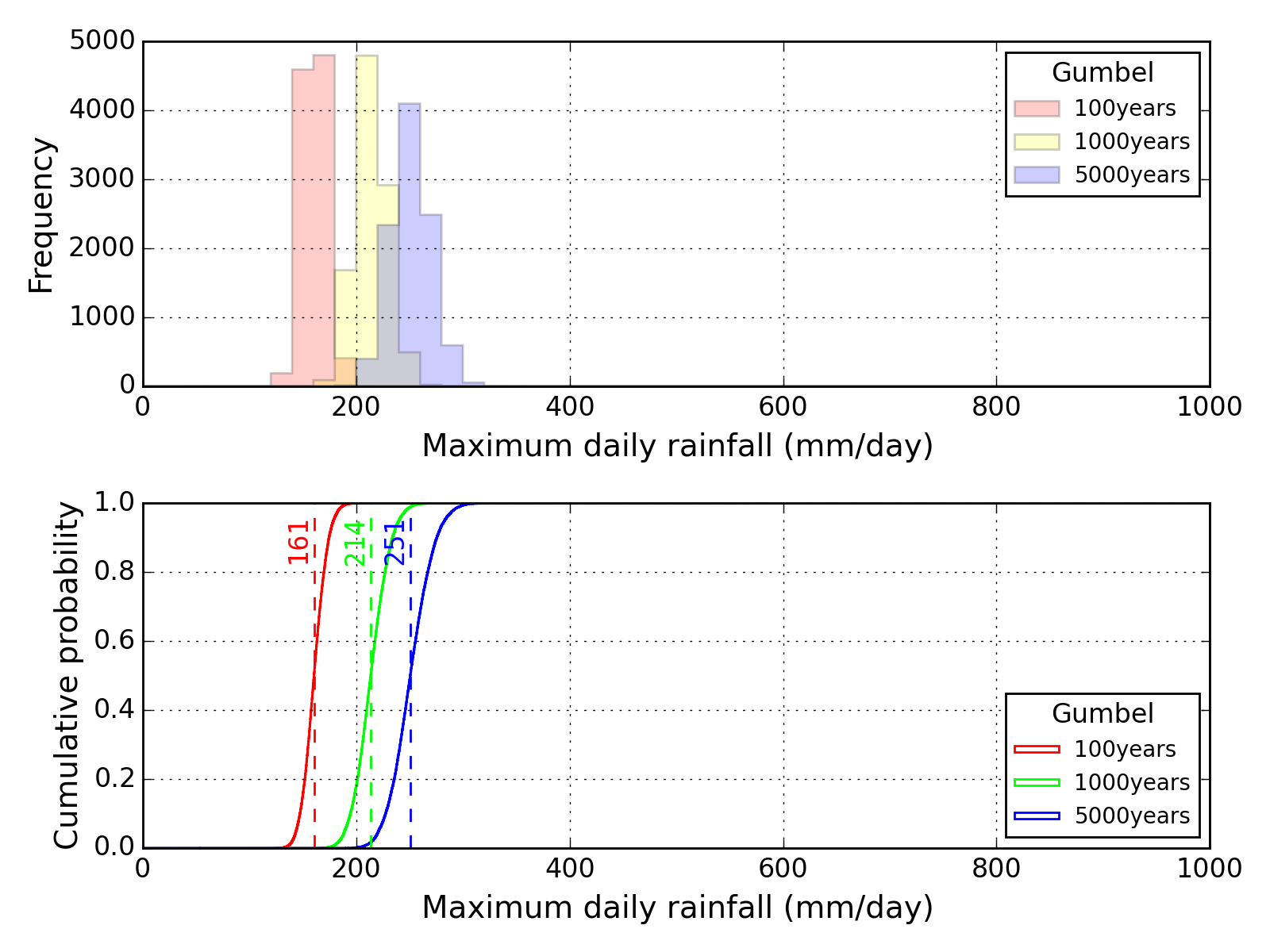
Retuen period
Return period
Return period is defined as follow:
\begin{equation}
T=\frac{1}{\mu (1-p)}
\end{equation}
| where, | $T$ | : return period or recurrence interval (year) |
| | $p$ | : non-exceedance probability for hydrological variable $x_p$ |
| | | $p=F(x_p) \qquad\qquad x_p=F^{-1}(p)$ |
| | | $x_p$ is often called quantile or $T$-year event. |
| | $\mu$ | : annual average number of occurrence of $X \geqq x_p$. |
Above is available for treatment of Peaks Over Threshold data (POT).
If we deal with Annual Maximum Series data (AMS), $\mu=1$ :
\begin{equation}
T=\frac{1}{1-p} \qquad p=1-\frac{1}{T}
\end{equation}
Reliability and Risk for $N$ years (for AMS)
\begin{align}
&P(X < x_T)_N=\left(1-\frac{1}{T}\right)^N & \text{Probability of non-exceedance for $N$ years}\\
&P(X\geqq x_T)_N=1-\left(1-\frac{1}{T}\right)^N & \text{Probability of exceedance at least once in $N$ years}
\end{align}
Sample calculation (for AMS)
| Return period (years) | T | 5 | 10 | 30 | 100 | 200 | 500 | 1000 | 5000 |
|---|
| Years considered | N | 5 | 5 | 5 | 10 | 20 | 50 | 100 | 500 |
| Non-exceedance probability | P | 0.328 | 0.590 | 0.844 | 0.904 | 0.905 | 0.905 | 0.905 | 0.905 |
Average, Variance, Skewness
\begin{align}
&\bar{x}=\frac{1}{N}\sum_{j=1}^N x_j &\text{Sample average}\\
&S^2=\frac{1}{N}\sum_{j=1}^N (x_j-\bar{x})^2 &\text{Sample variance}\\
&C_s=\frac{1}{N}\sum_{j=1}^N \left(\frac{x_j-\bar{x}}{S}\right)^3 &\text{Sample skewness}\\
&\hat{\sigma}^2=\frac{N}{N-1}S^2 &\text{Unbiased variance}\\
&\hat{\gamma}=\frac{\sqrt{N(N-1)}}{N-2}C_s &\text{Unbiased skewness}
\end{align}
PWM and L-Moments
Probabolity Weighted Moments (PWM) and L-Momets are adopted in a field of Hydrologic Frequency Analysis.
Although concept of order of data is not included in conventional use of average, variance and skewness, order statistics are adopted in use of PWM and L-Moments.
PWM for a population is defined below:
\begin{equation}
\beta_r=\int_0^1x F^r dF \qquad (r=0,1,2,\dots)
\end{equation}
and the relationship between PWM and L-Moments for a population is shown below:
\begin{align}
&\lambda_1=\beta_0 \\
&\lambda_2=2\beta_1-\beta_0 \\
&\lambda_3=6\beta_2-6\beta_1+\beta_0
\end{align}
PWM for a sample is shown below, and the relationship between PWM and L-Moments is same as the case for population.
\begin{align}
&b_0=\frac{1}{N}\sum_{j=1}^N x_{(j)} \\
&b_1=\frac{1}{N(N-1)}\sum_{j=1}^N (j-1) x_{(j)} \\
&b_2=\frac{1}{N(N-1)(N-2)}\sum_{j=1}^N (j-1)(j-2) x_{(j)}
\end{align}
where, $x_{(j)}$ is the $j$ th value in ascending order.
Plotting position formulas
A general formula for computing plotting position is defined as follow:
\begin{equation}
F[x_{(i)}]=\frac{i-\alpha}{N+1-2\alpha}
\end{equation}
| where | $N$ | : Number of sample |
| | $i$ | : Rank order in ascending order |
| | $x_{(i)}$ | : Value of sample with rank order $i$ in ascending order |
| | $F[x_{(i)}]$ | : Plotting position (like a non-exceedance probability) |
| | $\alpha$ | : Constant for a paticular plotting position formula ($\alpha=0\sim 1$) |
| Formula | Weibull | Blom | Cunnane | Gringorten | Hazen |
|---|
| $\alpha$ | 0 | 0.375 | 0.40 | 0.44 | 0.5 |
Probability Distribution Function for Hydrologic Frequency Analysis
Some Probability Distribution Functions for Hydrologic Frequency Analysis are enumerated below:
| Classification | Name of function | Number of
parameters |
|---|
Distribution of Block Maxima
such as Annual Maximum Series |
Generalized Extreme Value distribution | 3 |
Gumbel distribution | 2 |
Weibull distribution with 3 parameters | 3 |
SQRT exponential-type distribution of maximum | 2 |
| Distribution of Peaks Over Threshold |
Generalized Pareto distribution | 3 |
Exponential distribution | 2 |
| Empirical rule |
Normal distribution | 2 |
Log-Normal Distribution with 3 parameters | 3 |
Pearson type III distribution | 3 |
Log-Pearson type III distribution | 3 |
Probability Distribution Model
Normal distribution (N-distribution)
The parameter estimation method in the case of Hydrologic statistic $x$ following Normal distribution is shown below.
Probability Density Function
\begin{equation}
f(x)=\frac{1}{\sigma_x\sqrt{2\pi}}\cdot\exp\left[-\frac{1}{2}\left(\frac{x-\mu_x}{\sigma_x}\right)^2\right]
\end{equation}
Cumulative Distribution Function
\begin{equation}
F(x)=\Phi\left(\frac{x-\mu_x}{\sigma_x}\right)
\qquad \Phi(z)=\frac{1}{\sqrt{2\pi}}\int_{-\infty}^z\exp\left(-\frac{1}{2}t^2\right)dt
\end{equation}
Quantile $x_p$ for non-exceedance probability $p$
\begin{equation}
z=\frac{x-\mu_x}{\sigma_x} \qquad\rightarrow\qquad x=\mu_x+\sigma_x z
\end{equation}
\begin{equation}
x_p=\mu_x+\sigma_x z_p \qquad \text{$z_p$: $z$ value at $p=\Phi(z)$}
\end{equation}
Estimation of parameters using L-Moments
\begin{equation}
b_0=\frac{1}{N}\sum_{j=1}^N x_{(j)}
\qquad b_1=\frac{1}{N(N-1)}\sum_{j=1}^N (j-1) x_{(j)}
\end{equation}
where, $x_{(j)}$ is the $j$ th value in ascending order. $x_1$ means minimum value of $x_j$ .
The value of $\lambda_i$ can be calculated by deeming $b_i=\beta_i$ in above.
\begin{equation}
\lambda_1=\beta_0
\qquad \lambda_2=2\beta_1-\beta_0
\end{equation}
Parameters can be estimated using following relationship.
\begin{equation}
\begin{cases}
\mu_x=\lambda_1 \\
\sigma_x=\sqrt{\pi}\lambda_2
\end{cases}
\end{equation}
Log-Normal Distribution with 3 parameters (LN3-distribution)
The parameter estimation method in the case of Hydrologic statistic $x$ following Log-Normal distribution with 3 parameters is shown below.
Probability Density Function
\begin{equation}
f(x)=\frac{1}{(x-a)\sigma_y\sqrt{2\pi}}\cdot\exp\left\{-\frac{1}{2}\left[\frac{\ln(x-a)-\mu_y}{\sigma_y}\right]^2\right\}
\qquad y=\ln(x-a)
\end{equation}
Cumulative Distribution Function
\begin{equation}
F(x)=\Phi\left(\frac{\ln(x-a)-\mu_y}{\sigma_y}\right)
\qquad \Phi(z)=\frac{1}{\sqrt{2\pi}}\int_{-\infty}^z\exp\left(-\frac{1}{2}t^2\right)dt
\end{equation}
Quantile $x_p$ for non-exceedance probability $p$
\begin{equation}
z=\frac{\ln(x-a)-\mu_y}{\sigma_y} \qquad\rightarrow\qquad x=a+\exp(\mu_y+\sigma_y z)
\end{equation}
\begin{equation}
x_p=a+\exp(\mu_y+\sigma_y z_p) \qquad \text{$z_p$: value of $z$ at $p=\Phi(z)$}
\end{equation}
Estimation of parameters (Iwai method or Quantile method)
\begin{equation}
\begin{cases}
a=\cfrac{x_{(1)}\cdot x_{(N)}-x_m{}^2}{x_{(1)}+x_{(N)}-2 x_m} \qquad x_{(1)}+x_{(N)}-2x_m >0 \\
\mu_y=\cfrac{1}{N}\sum_{j=1}^N \ln(x_j-a) \\
\sigma_y{}^2=\cfrac{1}{N}\sum_{j=1}^N \left[\ln(x_j-a)-\mu_y\right]^2
\end{cases}
\end{equation}
where, $x_{(1)}$ is the minimum value of sample data, $x_{(N)}$ is the maximum value of sample data and $x_m$ is the median of sample data.
$x_{(j)}$ is $j$-th value of $x$ in ascending order.
Estimation of parameters (Moment method)
\begin{equation}
\qquad \bar{x}=\frac{1}{N}\sum_{j=1}^N x_j
\qquad S_x^2=\frac{1}{N}\sum_{j=1}^N (x_j-\bar{x})^2
\qquad C_{sx}=\frac{1}{N}\sum_{j=1}^N \left(\frac{x_j-\bar{x}}{S_x}\right)^3
\end{equation}
\begin{equation}
\mu_x=\bar{x}
\qquad \sigma_x=[N/(N-1)]^{1/2}S_x
\qquad \gamma_x=\frac{\sqrt{N(N-1)}}{N-2}C_{sx}
\end{equation}
(Reference)
To get the unbiased skewness $\gamma_x$ , the following formula for Log-Normal distribution by Bobee and Robitaille is adopted.
Note that $C_{sx}$ to the power of 3 is multiplied by $B$ .
\begin{gather}
\gamma_x=C_{sx}(A+B\cdot C_{sx}{}^3) \\
\text{where,} \qquad A=1.01+7.01/N+14.66/N^2 \qquad B=1.69/N+74.66/N^2
\end{gather}
The relationship between moments and parameters is shown below:
\begin{align}
&\mu_x=a+\exp(\mu_y)\cdot\exp(\sigma_y^2/2) \\
&\sigma_x=\exp(\mu_y)\sqrt{\exp(\sigma_y^2)\{\exp(\sigma_y^2)-1\}} \\
&\gamma_x=\{\exp(\sigma_y^2)+2\}\sqrt{\exp(\sigma_y^2)-1}
\end{align}
The parameters which we want to know are $\sigma_y$ , $\mu_y$ and $a$ in above equations.
The third equation in above is expressed as follow,
\begin{equation}
\gamma_x=\{\exp(\sigma_y^2)+2\}\sqrt{\exp(\sigma_y^2)-1} \Rightarrow x^3+3x^2-4-\gamma_x^2=0 \quad \text{where,}\quad x=\exp(\sigma_y^2)
\end{equation}
The real positive solution for above cubic equation can be obtained by Cardano's method as follow,
\begin{equation}
x=\left(\beta+\sqrt{\beta^2-1}\right)^{1/3}+\left(\beta-\sqrt{\beta^2-1}\right)^{1/3}-1 \quad \text{where,}\quad \beta=1+\frac{\gamma_x^2}{2}
\end{equation}
As a result, parameters can be estimated using following equations.
\begin{equation*}
\begin{cases}
\sigma_y=\sqrt{\ln(x)} & : \text{$x$ is a real positive solution of cubic equation $x^3+3x^2-4-\gamma_x^2=0$}\\
\mu_y=\ln\left(\cfrac{\sigma_x}{\sqrt{x(x-1)}}\right) \\
a=\mu_x-\exp(\mu_y)\cdot\exp(\sigma_y^2/2)
\end{cases}
\end{equation*}
Estimation of parameters (Trial method using single regression analysis)
Parameters can be obtain using following relationship.
\begin{equation}
z=\frac{\ln(x-a)-\mu_y}{\sigma_y} \quad\Rightarrow\quad z=A\cdot X+B
\end{equation}
\begin{equation}
X=\ln(x-a) \qquad A=\frac{1}{\sigma_y} \qquad B=-\frac{\mu_y}{\sigma_y}
\end{equation}
where, $z$ is a %-point of standard normal distribution.
It is calculated from the non-exceedance probability of $x$ .
Non-exceedance probability can be obtained using Protting position formula.
From above, following relationships are derived.
\begin{equation*}
\begin{cases}
a : \text{(selected value by trial single regression analysis)}\\
\mu_y=-\cfrac{B}{A} \\
\sigma_y=\cfrac{1}{A}
\end{cases}
\end{equation*}
$a$ is determind as a value in case that linear line has the maximum correlation coefficient.
The procedure to obtain the value of $a$ is shown below:
- Set the initial value of $a=x_{(1)}-\delta$ ( $\delta$ : small value).
- Repeat single regression analysis by reducing the value of $a$ .
- Select the value of $a$ when linear line has the maximum correlation coefficient.
Pearson type III distribution (P3-distribution)
The parameter estimation method in the case of Hydrologic statistic $x$ following Pearson type III distribution (Gamma distribution) is shown below.
Probability Density Function
\begin{equation}
f(x)=\frac{1}{|a|\cdot\Gamma(b)}\left(\frac{x-c}{a}\right)^{b-1}\cdot\exp\left(-\frac{x-c}{a}\right)
\qquad a > 0 : c\leqq x < \infty
\end{equation}
$c$ is a location parameter, $a$ is a scale parameter, $b$ is a shape parameter.
Cumulative Distribution Function
\begin{equation}
F(x)=G\left(\frac{x-c}{a}\right)
\qquad G(w)=\frac{1}{\Gamma(b)}\int_0^w t^{b-1}\exp(-t)dt \qquad (a>0)
\end{equation}
Quantile $x_p$ for non-exceedance probability $p$
\begin{equation}
w=\frac{x-c}{a} \qquad\rightarrow\qquad x=c+a w
\end{equation}
\begin{equation}
x_p=c+a w_p \qquad \text{$w_p$: Value od $w$ at $p=G(w)$}
\end{equation}
Estimation of parameters (Moment method)
\begin{equation}
\qquad \bar{x}=\frac{1}{N}\sum_{j=1}^N x_j
\qquad S_x^2=\frac{1}{N}\sum_{j=1}^N (x_j-\bar{x})^2
\qquad C_{sx}=\frac{1}{N}\sum_{j=1}^N \left(\frac{x_j-\bar{x}}{S_x}\right)^3
\end{equation}
\begin{equation}
\mu_x=\bar{x}
\qquad \sigma_x=[N/(N-1)]^{1/2}S_x
\qquad \gamma_x=\frac{\sqrt{N(N-1)}}{N-2}C_{sx}
\end{equation}
(Reference)
To get the unbiased skewness $\gamma_x$ , the following formula for Pearson type III distribution by Bobee and Robitaille is adopted.
Note that $C_{sx}$ to the power of 2 is multiplied by $B$ .
\begin{gather}
\gamma_x=C_{sx}(A+B\cdot C_{sx}{}^2) \\
\text{where,} \qquad A=1+6.51/N+20.2/N^2 \qquad B=1.48/N+6.77/N^2
\end{gather}
The relationship between moments and parameters is shown below:
\begin{equation}
\mu_x=c+a \cdot b \qquad
\sigma_x{}^2=a^2\cdot b \qquad
\gamma_x=\frac{2 a}{|a|\sqrt{b}}
\end{equation}
As a result, parameters can be estimated using following equations.
\begin{equation}
\begin{cases}
b=4/\gamma_x{}^2 \qquad (b>0) \\
a=\sigma_x/\sqrt{b} \qquad (\gamma_x < 0 \rightarrow a=-\sigma_x/\sqrt{b} < 0) \\
c=\mu_x-a b
\end{cases}
\end{equation}
Note that if $\gamma_x$ is less than $0$ ( $\gamma_x < 0$ ), $a$ shall be less than $0$ ( $a < 0$ ) and the value of $w_p$ is for the probability of $1-p$ .
If the absolute value of $\gamma_x$ is small, the same problem as Log-Pearson type III distribution may occur.
Log-Pearson type III distribution (LP3-distribution)
The parameter estimation method in the case of Hydrologic statistic $x$ following Log-Pearson type III distribution is shown below.
Probability Density Function
\begin{equation}
f(x)=\frac{1}{|a|\cdot\Gamma(b)\cdot x}\left(\frac{\ln x-c}{a}\right)^{b-1}\cdot\exp\left(-\frac{\ln x-c}{a}\right)
\qquad a > 0 : \exp(c) < x < \infty
\end{equation}
$c$ is a location parameter, $a$ is a scale parameter, $b$ is a shape parameter.
Cumulative Distribution Function
\begin{equation}
F(x)=G\left(\frac{\ln x-c}{a}\right)
\qquad G(w)=\frac{1}{\Gamma(b)}\int_0^w t^{b-1}\exp(-t)dt \qquad (a>0)
\end{equation}
Quantile $x_p$ for non-exceedance probability $p$
\begin{equation}
w=\frac{\ln x-c}{a} \qquad\rightarrow\qquad x=\exp(c+a w)
\end{equation}
\begin{equation}
x_p=\exp(c+a w_p) \qquad \text{$w_p$: the value of $w$ at $p=G(w)$}
\end{equation}
Estimation of parameters (Moment method)
\begin{equation}
y_j=\ln x_j
\qquad \bar{y}=\frac{1}{N}\sum_{j=1}^N y_j
\qquad S_y^2=\frac{1}{N}\sum_{j=1}^N (y_j-\bar{y})^2
\qquad C_{sy}=\frac{1}{N}\sum_{j=1}^N \left(\frac{y_j-\bar{y}}{S_y}\right)^3
\end{equation}
\begin{equation}
\mu_y=\bar{y}
\qquad \sigma_y=[N/(N-1)]^{1/2}S_y
\qquad \gamma_y=\frac{\sqrt{N(N-1)}}{N-2}C_{sy}
\end{equation}
(Reference)
To get the unbiased skewness $\gamma_x$ , the following formula for Pearson type III distribution by Bobee and Robitaille is adopted.
Note that $C_{sy}$ to the power of 2 is multiplied by $B$ .
\begin{gather}
\gamma_y=C_{sy}(A+B\cdot C_{sy}{}^2) \\
\text{where,} \qquad A=1+6.51/N+20.2/N^2 \qquad B=1.48/N+6.77/N^2
\end{gather}
The relationship between moments and parameters is shown below:
\begin{equation}
\mu_y=c+a \cdot b \qquad
\sigma_y{}^2=a^2\cdot b \qquad
\gamma_y=\frac{2 a}{|a|\sqrt{b}}
\end{equation}
As a result, parameters can be estimated using following equations.
\begin{equation}
\begin{cases}
b=4/\gamma_y{}^2 \qquad (b>0) \\
a=\sigma_y/\sqrt{b} \qquad (\gamma_y < 0 \rightarrow a=-\sigma_y/\sqrt{b} < 0) \\
c=\mu_y-a b
\end{cases}
\end{equation}
Note that if $\gamma_y$ is less than $0$ ( $\gamma_y < 0$ ), $a$ shall be less than $0$ and the value of $w_p$ is for the value of $1-p$ .
In the case of small absolute value of $\gamma_y$ , the value of $b$ becomes huge so that the converged value of percent point for Gamma distribution can not be obtained.
Therefore, if $b$ becomes huge value, quantile $x_p$ for non-exceedance probability $p$ can be calculated using Wilson-Hilferty transformation shown below.
\begin{equation}
x_p=\exp(\mu_y+\sigma_y\cdot K_p) \qquad
K_p=\frac{2}{\gamma_y}\left(1+\frac{\gamma_y z_p}{6}-\frac{\gamma_y{}^2}{36}\right)-\frac{2}{\gamma_y}
\end{equation}
where, $z_p$ is standard normal deviate following $N(0,1)$ .
If $b$ is greater than 10,000, it may be better to use Wilson-Hilferty transformation.
Even if skewness $\gamma_y$ is less than $0$ ( $\gamma_y < 0$ ), standard normal deviate $z_p$ shall be for the probability of $p$ ,
and it is not necessary to change the value of $\gamma_y$ to $|\gamma_y|$ (absolute value).
It means just calculated values of $p$ and $\gamma_y$ can be used for next calculation.
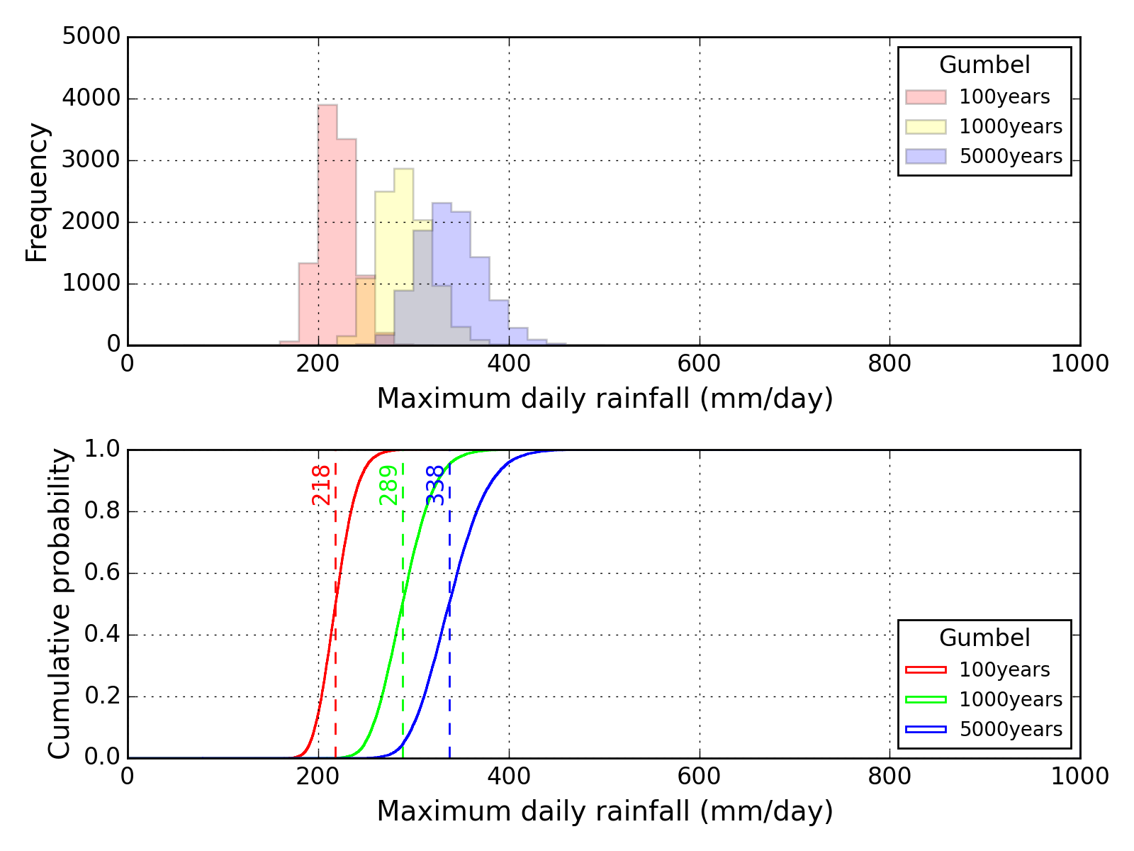
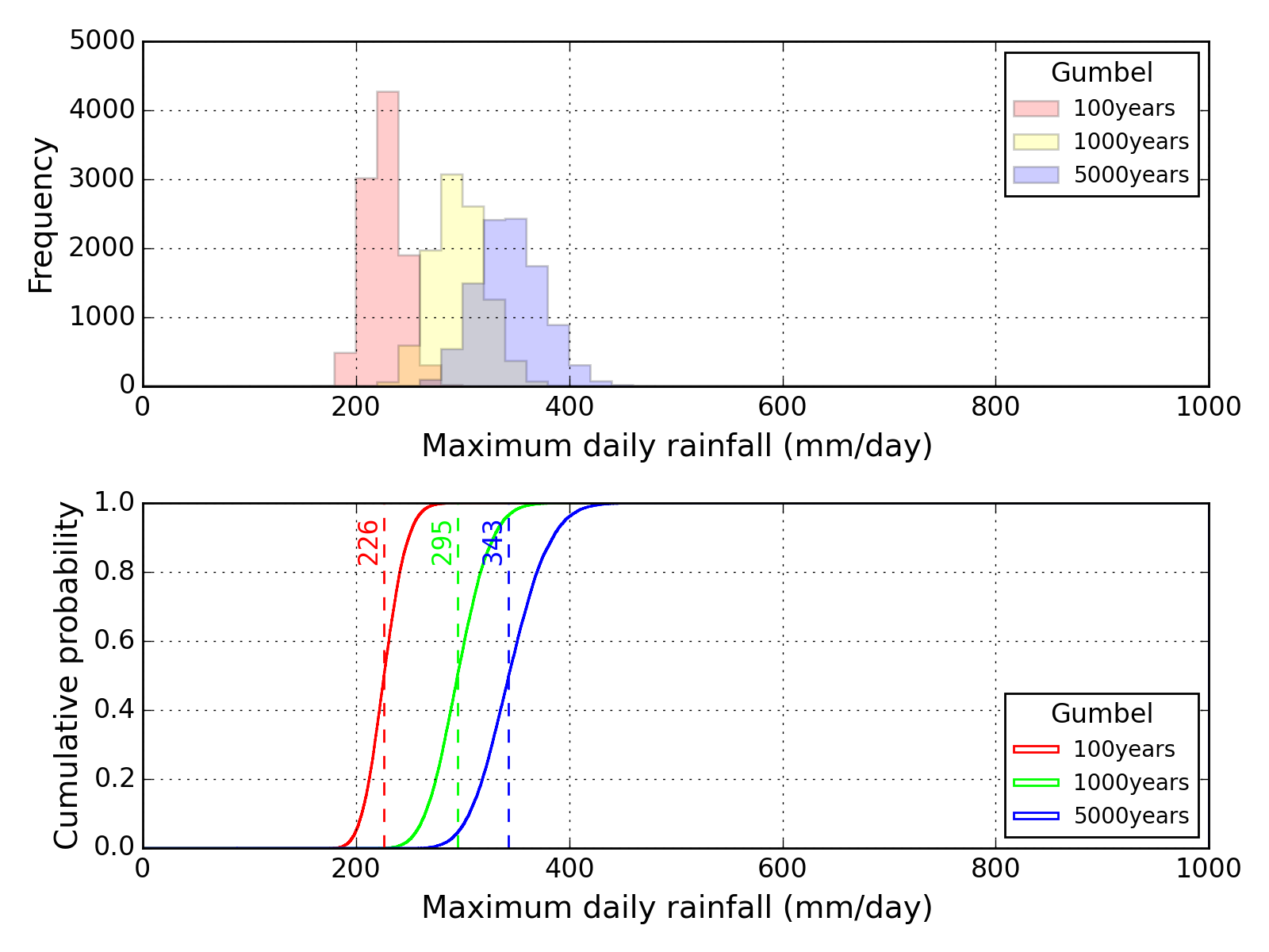
Gumbel distribution
The parameter estimation method in the case of Hydrologic statistic $x$ following Gumbel distribution is shown below.
Probability Density Function
\begin{equation}
f(x)=\frac{1}{a}\exp\left[-\frac{x-c}{a}-\exp\left(-\frac{x-c}{a}\right)\right] \qquad -\infty < x < \infty
\end{equation}
$c$ is a location parameter, $a$ is a scale parameter.
Cumulative Distribution Function
\begin{equation}
F(x)=\exp\left[-\exp\left(-\frac{x-c}{a}\right)\right]
\end{equation}
Quantile $x_p$ for non-exceedance probability $p$
\begin{equation}
p=\exp\left[-\exp\left(-\frac{x-c}{a}\right)\right] \qquad\rightarrow\qquad x=c-a\ln[-\ln(p)]
\end{equation}
\begin{equation}
x_p=c-a\ln[-\ln(p)]
\end{equation}
Estimation of parameters (L-moments method)
\begin{equation}
b_0=\frac{1}{N}\sum_{j=1}^N x_{(j)}
\qquad b_1=\frac{1}{N(N-1)}\sum_{j=1}^N (j-1) x_{(j)}
\end{equation}
where, $x_{(j)}$ is $j$ -th value of sample $x$ in ascending order.
It means that $x_{(1)}$ is the minimum value of sample data and $x_{(N)}$ is the maximum value of sample data.
The values of $\lambda_i$ can be calculated using following relationship by deeming $b_i=\beta_i$ .
\begin{equation}
\lambda_1=\beta_0
\qquad \lambda_2=2\beta_1-\beta_0
\end{equation}
Parameters can be estimated using following relationship between L-Moments and parameters.
\begin{equation}
\begin{cases}
a=\lambda_2/\ln 2 \\
c=\lambda_1-0.5772 a
\end{cases}
\end{equation}
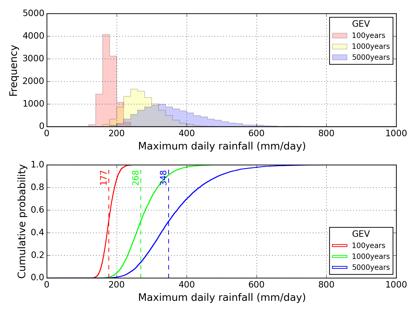
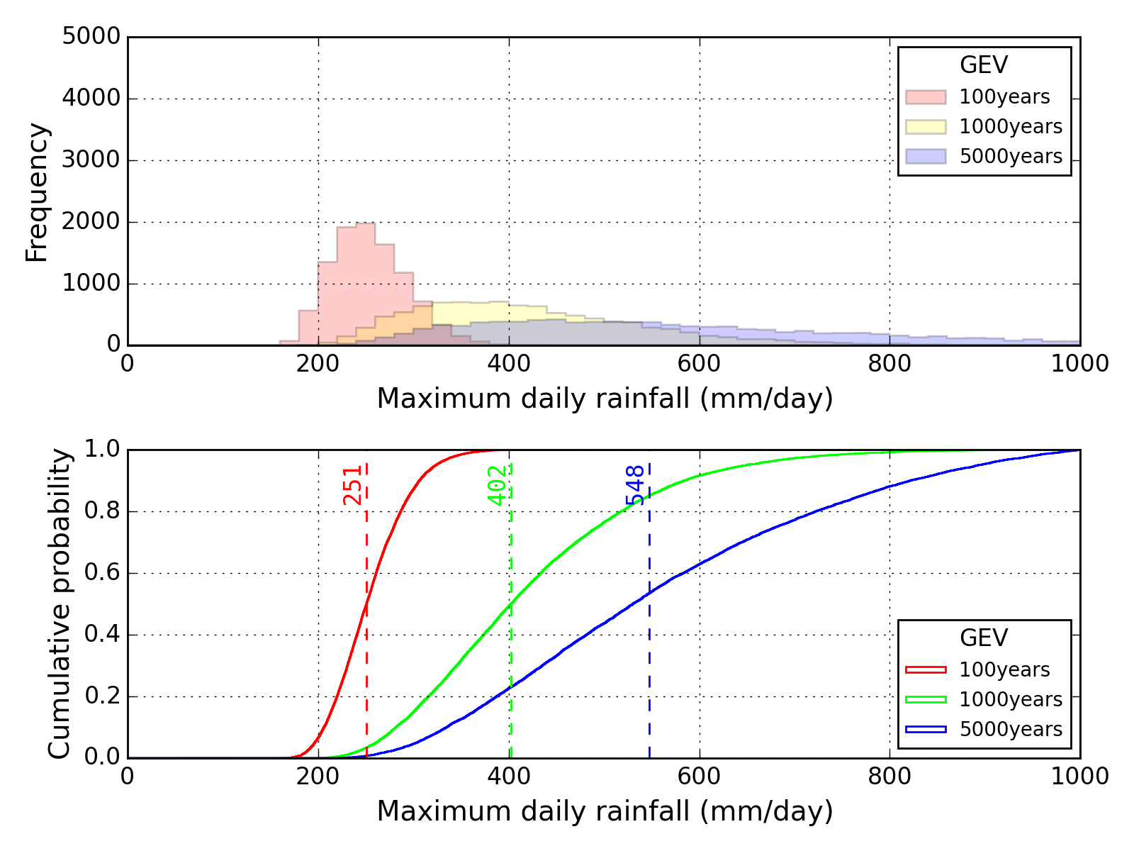
Generalized Extreme Value distribution (GEV-distribution)
The parameter estimation method in the case of Hydrologic statistic $x$ following Generalized Extreme Value distribution is shown below.
Gumbel distribution is the same as Generalized Extreme value distribution with $k=0$ .
Probability Density Function
\begin{equation}
f(x)=\frac{1}{a}\left(1-k\frac{x-c}{a}\right)^{1/k-1}\cdot\exp\left[-\left(1-k\frac{x-c}{a}\right)^{1/k}\right]
\qquad (k\neq 0)
\end{equation}
$c$ is a location parameter, $a$ is a scale parameter, $k$ is a shape parameter.
Cumulative Distribution Function
\begin{equation}
F(x)=\exp\left[-\left(1-k\frac{x-c}{a}\right)^{1/k}\right]
\qquad (k\neq 0)
\end{equation}
Quantile $x_p$ for non-exceedance probability $p$
\begin{equation}
p=\exp\left[-\left(1-k\frac{x-c}{a}\right)^{1/k}\right] \qquad\rightarrow\qquad x=c+\frac{a}{k}\cdot\left\{1-[-\ln(p)]^k\right\}
\end{equation}
\begin{equation}
x_p=c+\frac{a}{k}\cdot\left\{1-[-\ln(p)]^k\right\}
\end{equation}
Estimation of parameters (L-moments method)
\begin{equation}
b_0=\frac{1}{N}\sum_{j=1}^N x_{(j)}
\qquad b_1=\frac{1}{N(N-1)}\sum_{j=1}^N (j-1) x_{(j)}
\qquad b_2=\frac{1}{N(N-1)(N-2)}\sum_{j=1}^N (j-1)(j-2) x_{(j)}
\end{equation}
where, $x_{(j)}$ is $j$ -th value of sample $x$ in ascending order.
It means that $x_{(1)}$ is the minimum value of sample data and $x_{(N)}$ is the maximum value of sample data.
The values of $\lambda_i$ can be calculated using following relationship by deeming $b_i=\beta_i$ .
\begin{equation}
\lambda_1=\beta_0
\qquad \lambda_2=2\beta_1-\beta_0
\qquad \lambda_3=6\beta_2-6\beta_1+\beta_0
\end{equation}
Parameters can be estimated using following relationship between L-Moments and parameters.
\begin{equation}
\begin{cases}
k=7.8590d+2.9554d^2 \qquad \text{where, }
\qquad d=\cfrac{2\lambda_2}{\lambda_3+3\lambda_2}-\cfrac{\ln(2)}{\ln(3)} \\
a=\cfrac{k\lambda_2}{(1-2^{-k})\cdot\Gamma(1+k)} \\
c=\lambda_1-\cfrac{a}{k}\cdot\left[1-\Gamma(1+k)\right]
\end{cases}
\end{equation}
SQRT exponential-type distribution of maximum (SQRT-ET distribution)
The parameter estimation method in the case of Hydrologic statistic $x$ following SQRT exponential-type distribution of maximum is shown below.
Probability Density Function
\begin{equation}
f(x)=\frac{a b}{2}\exp\left[-\sqrt{bx}-a\left(1+\sqrt{bx}\right)\exp\left(-\sqrt{bx}\right)\right]
\qquad (x\geqq 0)
\end{equation}
Cumulative Distribution Function
\begin{equation}
F(x)=\exp\left[-a\left(1+\sqrt{bx}\right)\exp\left(-\sqrt{bx}\right)\right]
\qquad (x\geqq 0)
\end{equation}
Quantile $x_p$ for non-exceedance probability $p$
\begin{align}
&p=\exp\left[-a\left(1+\sqrt{bx}\right)\exp\left(-\sqrt{bx}\right)\right]
=\exp\left[-a(1+t_p)\exp(-t_p)\right] \qquad (t_p=\sqrt{b x}) \\
&\qquad\rightarrow\qquad x=\frac{t_p{}^2}{b} \qquad \ln(1+t_p)-t_p=\ln\left[-\frac{1}{a}\ln(p)\right]
\end{align}
\begin{equation}
x_p=\frac{t_p{}^2}{b}
\qquad \ln(1+t_p)-t_p=\ln\left[-\frac{1}{a}\ln(p)\right]
\end{equation}
(Reference) Calculation method of $t_p$
We define the function $g(t_p)$ as follow:
\begin{equation}
g(t_p)=\ln(1+t_p)-t_p-\ln\left[-\frac{1}{a}\ln(p)\right]
\end{equation}
Next we can get the differential of $g(t_p)$ as follow:
\begin{equation}
g'(t_p)=\frac{1}{1+t_p}-1
\end{equation}
So we can know that function $g(t_p)$ is a monotone decreasing function because the value of $g'(t_p)$ is negative for valid $t_p$ .
And we can obtain the value of $t_p$ at $g(t_p)=0$ using Newton-Raphson method shown below.
\begin{equation}
t_{p(n+1)}=t_{p(n)}-\frac{g(t_{p(n)})}{g'(t_{p(n)})} \qquad \text{$(n)$: counter for iterative calculation}
\end{equation}
Regarding an initial value of $t_p$ , it is convenient to use the value of $t_p=\sqrt{b\cdot x_{max}}$ ,
because we want to know the value of $x_p$ at the heigher range of non-exceedance probability of $p$ .
Estimation of parameters (Maximum Likelihood Method)
Parameters $a$ and $b$ are determined so that a log-likelihood function $L$ shown below has the maximum value.
\begin{align}
&L(a,b)=\sum_{j=1}^N \ln f(x_j) \notag \\
&=N\ln a+N\ln b-N\ln 2-\sum_{j=1}^N \sqrt{b x_j}-a\left[\sum_{j=1}^N \exp\left(-\sqrt{bx_j}\right)+\sum_{j=1}^N \sqrt{b x_j}\exp\left(-\sqrt{b x_j}\right)\right]
\end{align}
From the condition that partial differential of $L$ by $b$ becomes 0, $a$ can be expressed as a function of $b$ .
We define this temporary value equals to $a_1$ .
\begin{equation}
\frac{\partial L}{\partial b}=0 \qquad\rightarrow\qquad a=\cfrac{\sum_{j=1}^N \sqrt{b x_j}-2N}{\sum_{j=1}^N (b x_j)\exp\left(-\sqrt{b x_j}\right)}=a_1
\end{equation}
Next, from the condition that partial differential of $L$ by $a$ becomes 0, $a$ can be expressed as a function of $b$ .
We define this temporary value equals to $a_2$ .
\begin{equation}
\frac{\partial L}{\partial a}=0 \qquad\rightarrow\qquad a=\cfrac{N}{\sum_{j=1}^N \exp\left(-\sqrt{bx_j}\right)+\sum_{j=1}^N \sqrt{b x_j}\exp\left(-\sqrt{b x_j}\right)}=a_2
\end{equation}
Since $L$ has the maximum value at the condition of $a_1=a_2$ , the value of $b$ can be obtained using bisection method,
where the equation for bisection method is $h(b)=a_1(b)-a_2(b)=0$ .
Note that $a_2 > 0$ is everytime true, but $b$ shall satisfy the following condition for ensureing $a_1 > 0$ .
\begin{equation}
a_1>0 \qquad\rightarrow\qquad b>\left(\frac{2 N}{\sum_{j=1}^N \sqrt{x_j}}\right)^2
\end{equation}
Sample program by C language is shown below.
/* Bisection method */
b1=bb;                        /* Set the value of b1 (condition: a1>0) */
b2=b1+0.5;                    /* Set the value of b2 as the value of b1+0.5 */
bb=0.5*(b1+b2);               /* Set the intermediate value of bb */
f1=FSQR(nd,datax,b1,&a1,&a2); /* Get the value of h(b1) */
f2=FSQR(nd,datax,b2,&a1,&a2); /* Get the value of h(b2) */
ff=FSQR(nd,datax,bb,&a1,&a2); /* Get the value of h(bb) */
do{                           /* Loop for iterative calculation */
    if(f1*ff<0.0)b2=bb;
    if(ff*f2<0.0)b1=bb;
    if(ff==0.0)break;
    if(0.0<f1*ff&&0.0<ff*f2){b1=b2;b2=b1+0.5;} /* Technique for searching the solution. */
    bb=0.5*(b1+b2);
    f1=FSQR(nd,datax,b1,&a1,&a2);
    f2=FSQR(nd,datax,b2,&a1,&a2);
    ff=FSQR(nd,datax,bb,&a1,&a2);
}while(0.001<fabs(a1-a2));    /* Criteria for judgement of convergence: |h(b)|<0.001 */
|
Weibull distribution with 3 parameters
The parameter estimation method in the case of Hydrologic statistic $x$ following Weibull distribution with 3 parameters is shown below.
Probability Density Function
\begin{equation}
f(x)=\frac{k}{a}\left(\frac{x-c}{a}\right)^{k-1}\exp{\left[-\left(\frac{x-c}{a}\right)^k\right]}
\qquad (k\neq 0)
\end{equation}
$c$ is a location parameter, $a$ is a scale parameter, $k$ is a shape parameter.
Cumulative Distribution Function
\begin{equation}
F(x)=1-\exp\left[-\left(\frac{x-c}{a}\right)^k\right]
\qquad (k\neq 0)
\end{equation}
Quantile $x_p$ for non-exceedance probability $p$
\begin{equation}
1-p=\exp\left[-\left(\frac{x-c}{a}\right)^k\right] \qquad\rightarrow\qquad x=c+a[-\ln{(1-p)}]^{1/k}
\end{equation}
\begin{equation}
x_p=c+a[-\ln{(1-p)}]^{1/k}
\end{equation}
Estimation of parameters (L-moments method by Goda *)
\begin{equation}
b_0=\frac{1}{N}\sum_{j=1}^N x_{(j)}
\qquad b_1=\frac{1}{N(N-1)}\sum_{j=1}^N (j-1) x_{(j)}
\qquad b_2=\frac{1}{N(N-1)(N-2)}\sum_{j=1}^N (j-1)(j-2) x_{(j)}
\end{equation}
where, $x_{(j)}$ is $j$ -th value of sample $x$ in ascending order.
It means that $x_{(1)}$ is the minimum value of sample data and $x_{(N)}$ is the maximum value of sample data.
The values of $\lambda_i$ can be calculated using following relationship by deeming $b_i=\beta_i$ .
\begin{equation}
\lambda_1=\beta_0
\qquad \lambda_2=2\beta_1-\beta_0
\qquad \lambda_3=6\beta_2-6\beta_1+\beta_0
\end{equation}
Parameters can be estimated using following relationship between L-Moments and parameters.
\begin{equation}
\begin{cases}
k=285.3\tau^6-658.6\tau^5+622.8\tau^4-317.2\tau^3+98.52\tau^2-21.256\tau+3.5160
\qquad \text{where} \quad \tau=\lambda_3/\lambda_2 \\
a=\cfrac{\lambda_2}{(1-2^{-1/k})\cdot\Gamma(1+1/k)} \\
c=\lambda_1-a\cdot\Gamma(1+1/k)
\end{cases}
\end{equation}
(Reference)
*) https://www.jstage.jst.go.jp/article/kaigan/65/1/65_1_161/_pdf,
''Use of L-moments Method for Extreme Statistics of Storm Wave Heights''
(auther: Yoshimi GODA, Masanobu KUDAKA and Hiroyasu KAWAI)
For the item of Weibull distribution in the Table-2 on above paper:
Although $k$ is the function of $\lambda_3$ in this table, I think $\tau_3=\lambda3/\lambda_2$ is correct.
In addition, although denominator of $A$ includes $k$ , I think this is miss type.
Estimation of parameters (Maximum Likelihood Method)
Since 3 parameters are included in this problem, following procedure can be adopted.
- First, to estimate location parameter $c$ using plotting position formula. As a result, $c$ becomes known parameter.
- Second, to estimate shape parameter $k$ and scale parameter $a$ using known parameter of $c$ . As a calculation method, Maximum Likelihood Method can be used.
(I) Estimation of location parameter $c$
Non-exceedance probability $F(x)$ of sample $x$ can be estimated using plotting position formula.
Note that sample data shall be sorted order in ascending to use plotting position formula.
Following equation is obtained by transforming Cumulative Distribution Function.
\begin{equation}
1-F(x)=\exp\left[-\left(\frac{x-c}{a}\right)^k\right]
\end{equation}
From above, following equation can be obtained as a logarithm of 2 times.
\begin{equation}
\ln\{-\ln[1-F(x)]\}=k \ln(x-c)-k \ln a \qquad\rightarrow\qquad Y=A\cdot X+B
\end{equation}
Next, $k$ and $a$ can be obtained using following equations based on single regression analysis.
\begin{gather}
Y_i=\ln\{-\ln[1-F(x_i)]\} \qquad \qquad X_i=\ln(x_i-c) \\
A=\frac{N \sum X_i Y_i-\sum X\cdot\sum Y_i}{N \sum X_i{}^2-(\sum X_i)^2}
\qquad \qquad
B=\frac{\sum X_i{}^2\cdot \sum Y_i-\sum X_i\cdot\sum X_i Y_i}{N \sum X_i{}^2-(\sum X_i)^2} \\
r=\frac{N \sum X_i Y_i-\sum X_i\cdot\sum Y_i}{\sqrt{[N \sum X_i^2-(\sum X_i)^2]\cdot [N \sum Y_i{}^2-(\sum Y_i)^2]}}
\end{gather}
\begin{equation}
k=A \qquad \qquad a=\exp(-B/A)
\end{equation}
where, $N$ is sample number.
Since $c$ is unknown value in above equations,
it is necessary to carry out the trial calculation to get the optimal value of $c$ which gives maximum value of correlation coefficient $r$ by simple regression analysis.
In this stage, temporary values of $k$ , $a$ and $c$ are obtained.
However, it is desirable to carry out additional calculation in order to get the more certain values.
In next stage, the condition is that $c$ is fixed and $k$ and $a$ are unknown values.
(II) Estimation of shape parameter $k$ and scale parameter $a$
By setting $t=x-c$ , following equation is obtained, where $c$ is already fixed (known parameter).
\begin{equation}
f(t)=\frac{k}{a}\left(\frac{t}{a}\right)^{k-1}\exp{\left[-\left(\frac{t}{a}\right)^k\right]}
\end{equation}
Using log likelihood function for above equation $L=\sum_{i=1}^N \ln f(t_i)$ , $k$ and $a$ can be estimated by Newton-Raphson method.
As an initial value of $k$ , obtained value in previous step can be used.
\begin{align}
&\frac{\partial L}{\partial k}=0 &\rightarrow\qquad &\frac{1}{k}+\cfrac{\sum_{i=1}^N \ln{t_i}}{N}-\cfrac{\sum_{i=1}^N [(\ln{t_i})\cdot t_i{}^k]}{\sum_{i=1}^N t_i{}^k}=0 \\
&\frac{\partial L}{\partial a}=0 &\rightarrow\qquad &a=\left(\cfrac{\sum_{i=1}^N t_i{}^k}{N}\right)^{1/k}
\end{align}
\begin{equation}
g(k)=\frac{1}{k}+\frac{T_0}{N}-\frac{T_2(k)}{T_1(k)} \qquad\qquad
g'(k)=-\frac{1}{k^2}-\frac{T_3(k)\cdot T_1(k)-[T_2(k)]^2}{[T_1(k)]^2}
\end{equation}
\begin{equation}
T_0=\sum_{i=1}^N \ln{t_i} \qquad
T_1(k)=\sum_{i=1}^N t_i{}^k \qquad
T_2(k)=\sum_{i=1}^N [\ln{t_i}\cdot t_i{}^k] \qquad
T_3(k)=\sum_{i=1}^N [\ln{t_i}\cdot \ln{t_i}\cdot t_i{}^k]
\end{equation}
Iterative calculation using following equation shall be carried out untill getting converged value of $k$ , where $n$ is a counter for iterative calculation.
\begin{equation}
k_{n+1}=k_n-\frac{g(k_n)}{g'(k_n)}
\end{equation}
If the value of $k$ is defined, the value of $a$ also can be defined using below.
\begin{equation}
a=\left(\cfrac{\sum_{i=1}^N t_i{}^k}{N}\right)^{1/k}
\end{equation}
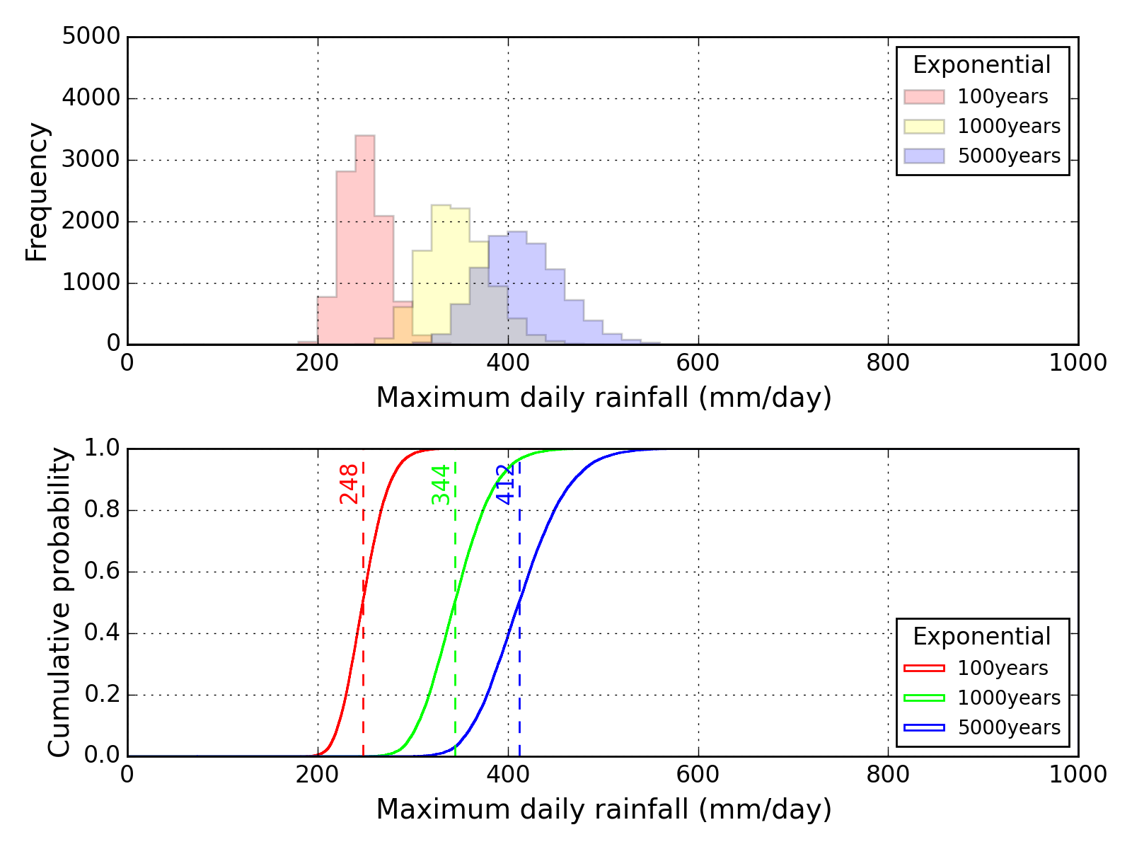
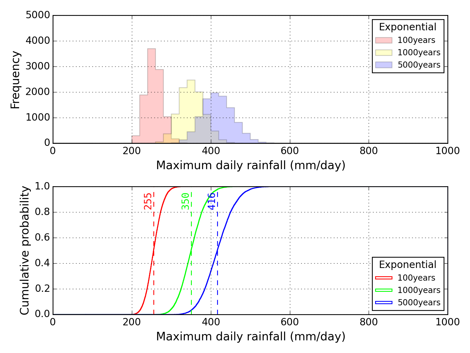
Exponential distribution
The parameter estimation method in the case of Hydrologic statistic $x$ following Exponential distribution is shown below.
Probability Density Function
\begin{equation}
f(x)=\frac{1}{a}\exp\left(-\frac{x-c}{a}\right)
\end{equation}
$c$ is a location parameter, $a$ is a scale parameter.
Cumulative Distribution Function
\begin{equation}
F(x)=1-\exp\left(-\frac{x-c}{a}\right)
\end{equation}
Quantile $x_p$ for non-exceedance probability $p$
\begin{equation}
p=1-\exp\left(-\frac{x-c}{a}\right)\qquad\rightarrow\qquad x=c-a\ln(1-p)
\end{equation}
\begin{equation}
x_p=c-a\ln(1-p)
\end{equation}
Estimation of parameters (L-moments method)
\begin{equation}
b_0=\frac{1}{N}\sum_{j=1}^N x_{(j)}
\qquad b_1=\frac{1}{N(N-1)}\sum_{j=1}^N (j-1) x_{(j)}
\end{equation}
where, $x_{(j)}$ is $j$ -th value of sample $x$ in ascending order.
It means that $x_{(1)}$ is the minimum value of sample data and $x_{(N)}$ is the maximum value of sample data.
The values of $\lambda_i$ can be calculated using following relationship by deeming $b_i=\beta_i$ .
\begin{equation}
\lambda_1=\beta_0
\qquad \lambda_2=2\beta_1-\beta_0
\end{equation}
Parameters can be estimated using following relationship between L-Moments and parameters.
\begin{equation}
\begin{cases}
a=2\lambda_2 \\
c=\lambda_1-a
\end{cases}
\end{equation}
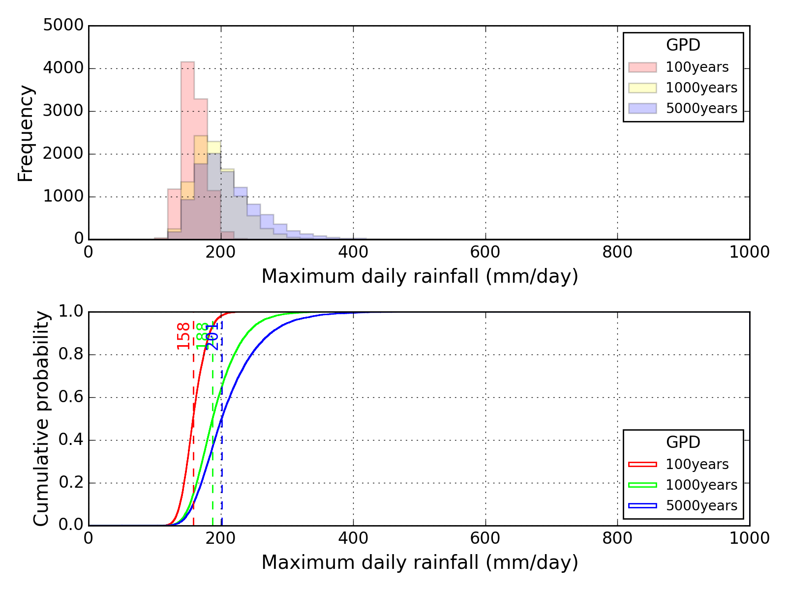
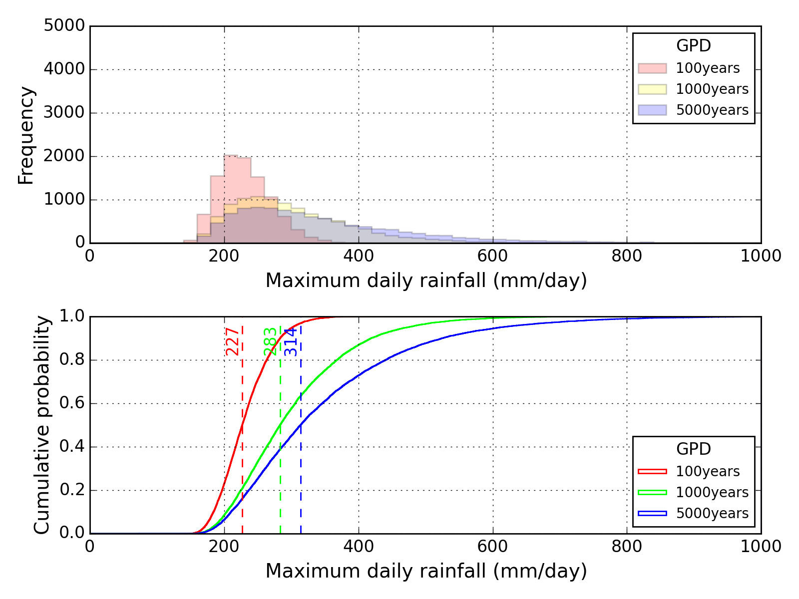
Generalized Pareto distribution (GPD)
The parameter estimation method in the case of Hydrologic statistic $x$ following Generalized pareto distribution is shown below.
Exponential distribution is the same as Generalized Pareto distribution with $k=0$ .
Probability Density Function
\begin{equation}
f(x)=\frac{1}{a}\left(1-k\frac{x-c}{a}\right)^{1/k-1} \qquad (k\neq 0)
\end{equation}
$c$ is a location parameter, $a$ is a scale parameter, $k$ is a shape parameter.
Cumulative Distribution Function
\begin{equation}
F(x)=1-\left(1-k\frac{x-c}{a}\right)^{1/k}
\qquad (k\neq 0)
\end{equation}
Quantile $x_p$ for non-exceedance probability $p$
\begin{equation}
p=1-\left(1-k\frac{x-c}{a}\right)^{1/k}\qquad\rightarrow\qquad x=c+\frac{a}{k}\left\{1-(1-p)^k\right\}
\end{equation}
\begin{equation}
x_p=c+\frac{a}{k}\cdot\left\{1-(1-p)^k\right\}
\end{equation}
Estimation of parameters (L-moments method)
\begin{equation}
b_0=\frac{1}{N}\sum_{j=1}^N x_{(j)}
\qquad b_1=\frac{1}{N(N-1)}\sum_{j=1}^N (j-1) x_{(j)}
\qquad b_2=\frac{1}{N(N-1)(N-2)}\sum_{j=1}^N (j-1)(j-2) x_{(j)}
\end{equation}
where, $x_{(j)}$ is $j$ -th value of sample $x$ in ascending order.
It means that $x_{(1)}$ is the minimum value of sample data and $x_{(N)}$ is the maximum value of sample data.
The values of $\lambda_i$ can be calculated using following relationship by deeming $b_i=\beta_i$ .
\begin{equation}
\lambda_1=\beta_0
\qquad \lambda_2=2\beta_1-\beta_0
\qquad \lambda_3=6\beta_2-6\beta_1+\beta_0
\end{equation}
Parameters can be estimated using following relationship between L-Moments and parameters.
\begin{equation}
\begin{cases}
k=\cfrac{\lambda_2-3\lambda_3}{\lambda_2+\lambda_3} \\
a=(1+k)(2+k)\lambda_2 \\
c=\lambda_1-(2+k)\lambda_2
\end{cases}
\end{equation}
Confirmation of fitness
Correlation Coefficient
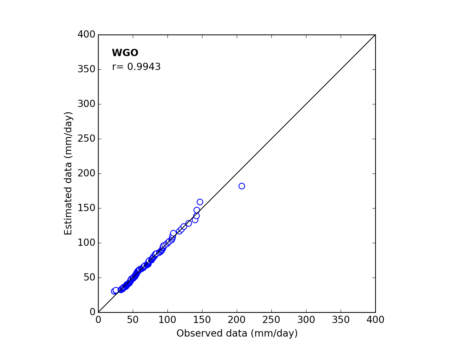
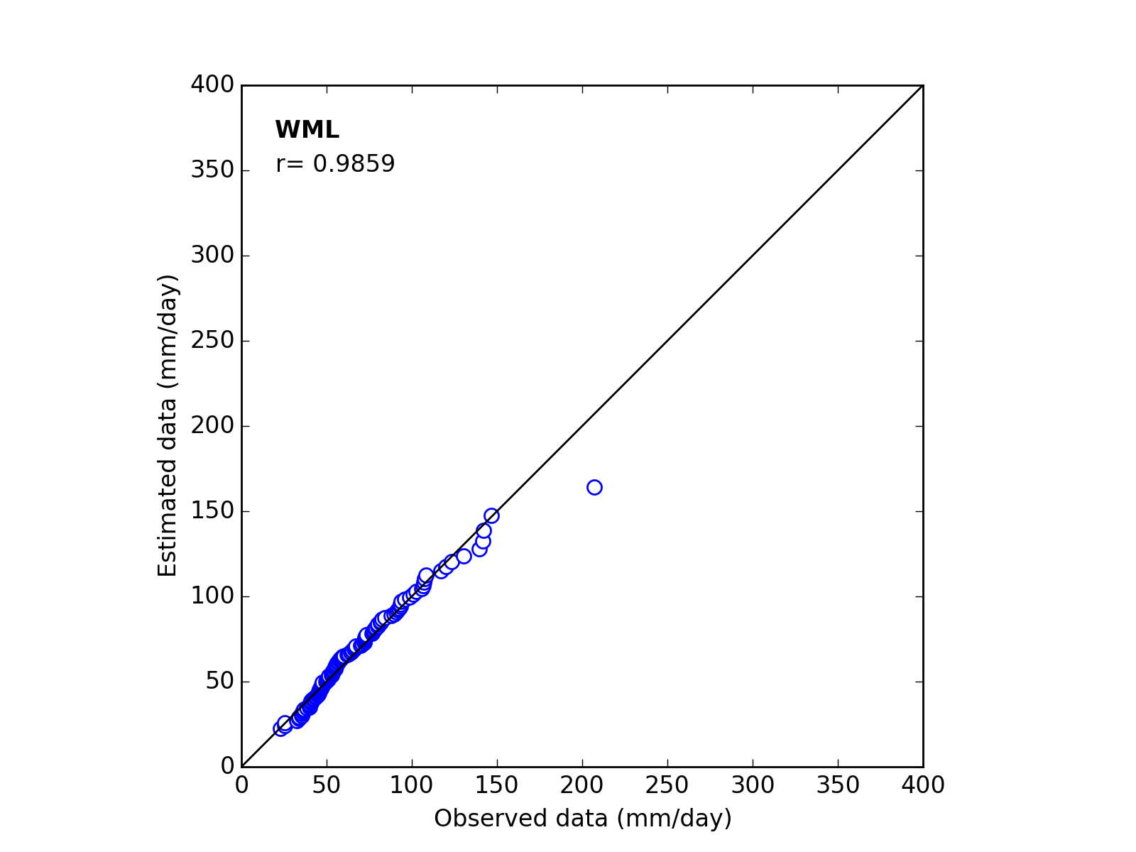
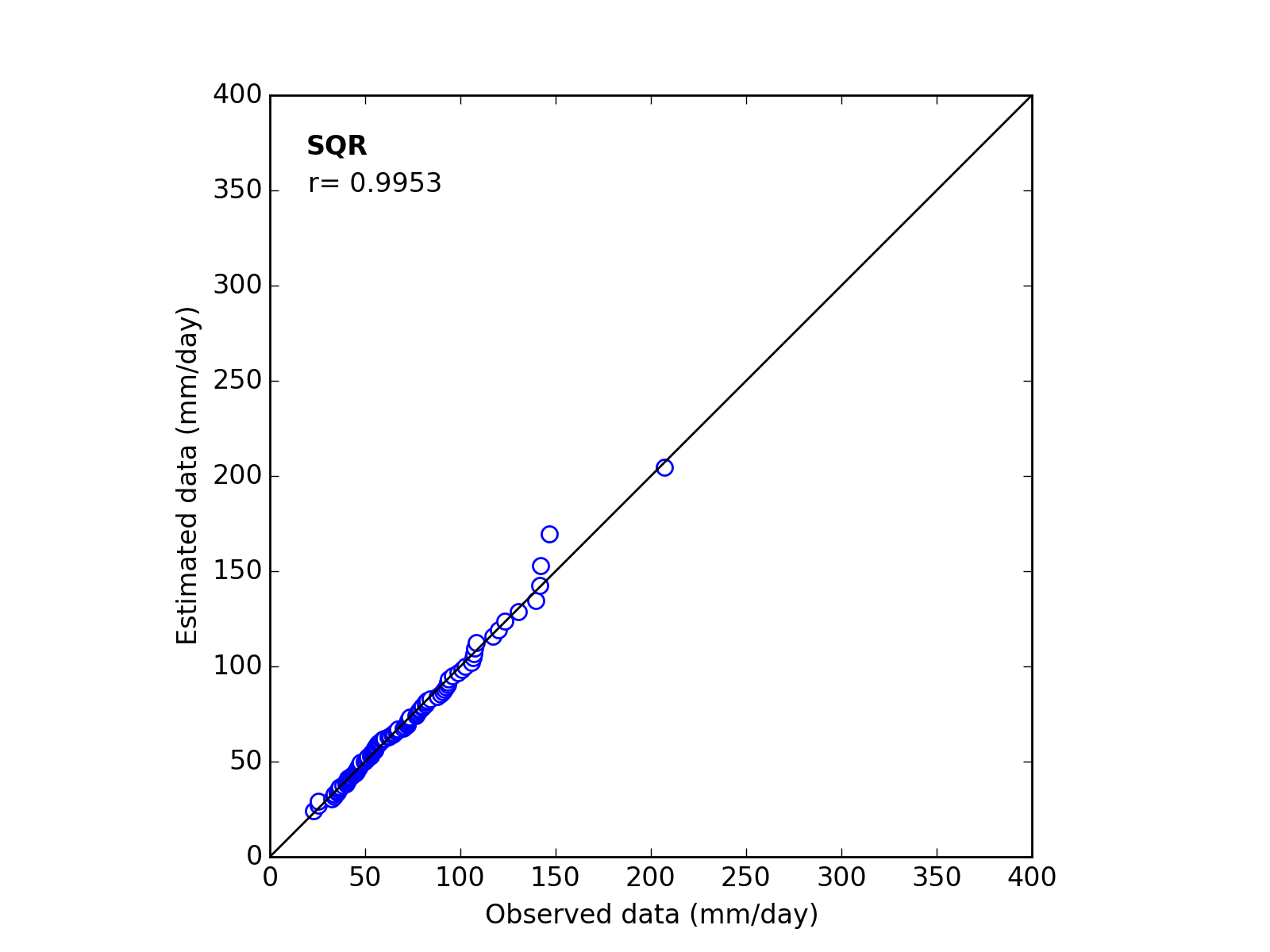
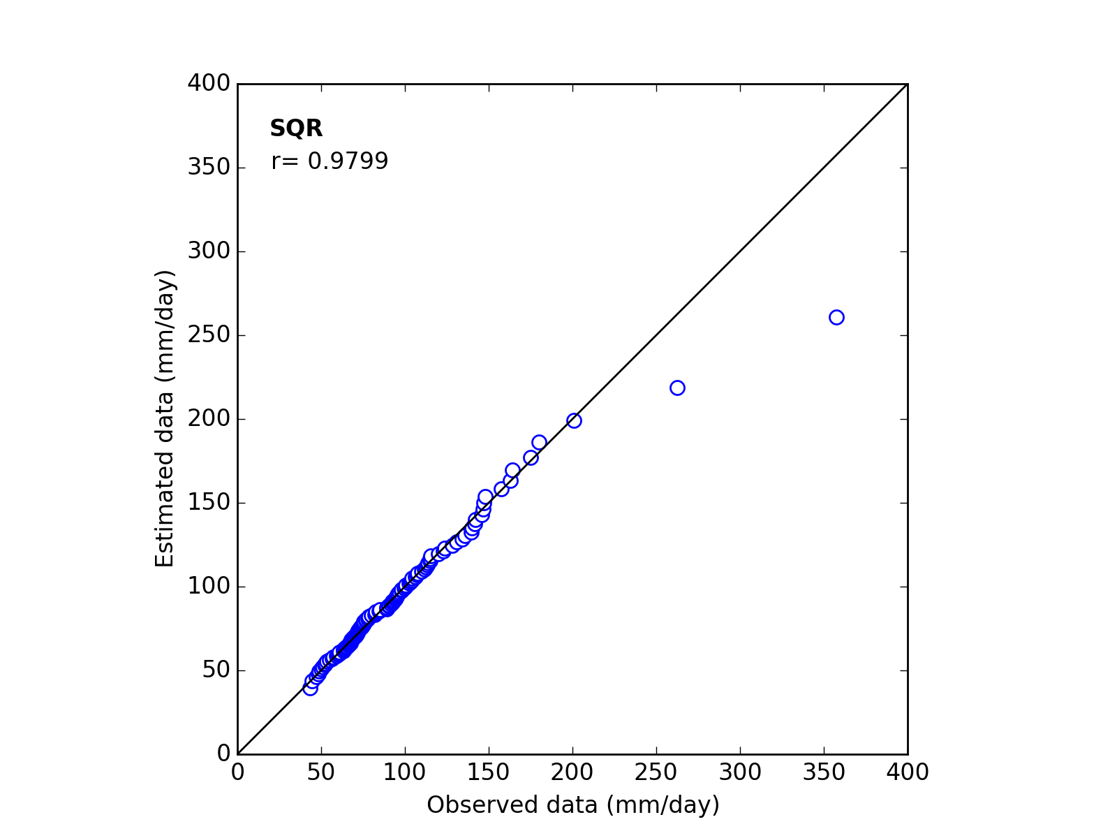
In order to confirm the fitness of the selected probability distribution model,
Q-Q (quantile-quantile) plot is used and the correlation coefficient is written in the graph.
In this section, equations to calculate the correlation coefficient is shown.
\begin{equation*}
r=\frac{N \sum X_i Y_i-\sum X_i\cdot\sum Y_i}{\sqrt{[N \sum X_i^2-(\sum X_i)^2]\cdot [N \sum Y_i{}^2-(\sum Y_i)^2]}}
\end{equation*}
| where, | $r$ | : correlation coefficient |
| | $N$ | : number of a sample |
| | $X_i$ | : observed data |
| | $Y_i$ | : calculated data using probability distribution model |
SLSC
\begin{equation}
\text{SLSC}=\cfrac{\sqrt{\cfrac{1}{N}\cdot\sum_{j=1}^{j=N}(s_j-r_j)}}{|r_{0.99}-r_{0.01}|}
\end{equation}
| $s_i$ | : Normalized variable by parameters |
| $r_i$ | : Normalized variable by Plotting position formula |
| $r_{0.99}$ | : Normalized value corresponding to the non-exceedance probability of 99% |
| $r_{0.01}$ | : Normalized value corresponding to the non-exceedance probability of 1% |
| Distribution | Si | ri |
|---|
| LN3 | $\cfrac{\ln(x_i-a)-\mu_y}{\sigma_y}$ | $qnorm(p_i)$
(%-point of SND) |
| LP3 | $\cfrac{\ln x_i-c}{a}$ | $qgamma(p_i,shape=b,rate=1)$
(%-point of Gamma Distribution) |
| Gumbel | $\exp\left(-\cfrac{x_i-c}{a}\right)$ | $-\ln(p_i)$ |
| GEV | $\left(1-k\cfrac{x_i-c}{a}\right)^{1/k}$ | $-\ln(p_i)$ |
| SQRT-ET | $a\cdot\exp\{\ln(1+\sqrt{b x_i})-\sqrt{b x_i}\}$ | $-\ln(p_i)$ |
| Weibull | $\left(\cfrac{x_i-c}{a}\right)^k$ | $-\ln(1-p_i)$ |
| Exponential | $\cfrac{x_i-c}{a}$ | $-\ln(1-p_i)$ |
| GPD | $-\cfrac{1}{k}\cdot\ln\left(1-k\cdot\cfrac{x_i-c}{a}\right)$ | $-\ln(1-p_i)$ |
Statistical estimation by Jackknife method
The method to obtain the bias-corrected estimate and standard error by Jackknife method is shown in this section.
The procedure by Jackknife method is shown below.
- (1) Obtain the statistic estimate $\hat{\theta}$ using ovserved sample $X=(x_1,x_2,\cdots,x_N)$ with sample size of $N$ .
- (2) Obtain the statistic estimate $\hat{\theta}_{(i)}$ using sample $X_i=(x_1,x_2,\cdots,x_{i-1},x_{i+1},\cdots,x_N)$ with sample size of $N-1$ .
In the dataset $X_i$ , $i$ -th data $x_i$ is removed.
- (3) By repeating above, dataset $(\hat{\theta}_{(1)},\cdots,\hat{\theta}_{(N)})$ with the sample size of $N$ can be obtain.\\
Next, obtain the average of dataset $(\hat{\theta}_{(1)},\cdots,\hat{\theta}_{(N)})$ .
\begin{equation}
\hat{\theta}_{(\cdot)}=\frac{1}{N}\sum_{i=1}^N \hat{\theta}_{(i)}
\end{equation}
- (4) Obtain {\bfseries the bias-corrected jackknife estimate} using following equation.
\begin{equation}
\bar{\theta}=N\cdot\hat{\theta}-(N-1)\cdot\hat{\theta}_{(\cdot)}
\end{equation}
where, $\hat{\theta}$ is the value obtained from step\MARU{1} using original sample $X=(x_1,x_2,\cdots,x_N)$ with sample size of $N$ ,
and $\hat{\theta}_{(\cdot)}$ is the average value obtained from step\MARU{2} and \MARU{3} using re-sampled dataset $X_i=(x_1,x_2,\cdots,x_{i-1},x_{i+1},\cdots,x_N)$ with sample size of $N-1$ .
- (5) Finaly, {\bfseries the standard error (SE)} of $\theta$ can be obtained using following equation.
\begin{equation}
(SE)=\sqrt{\cfrac{N-1}{N}\sum_{i=1}^N \left(\hat{\theta}_{(i)}-\hat{\theta}_{(\cdot)}\right)^2}
\end{equation}
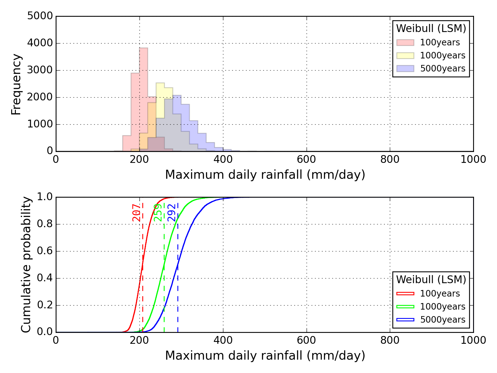
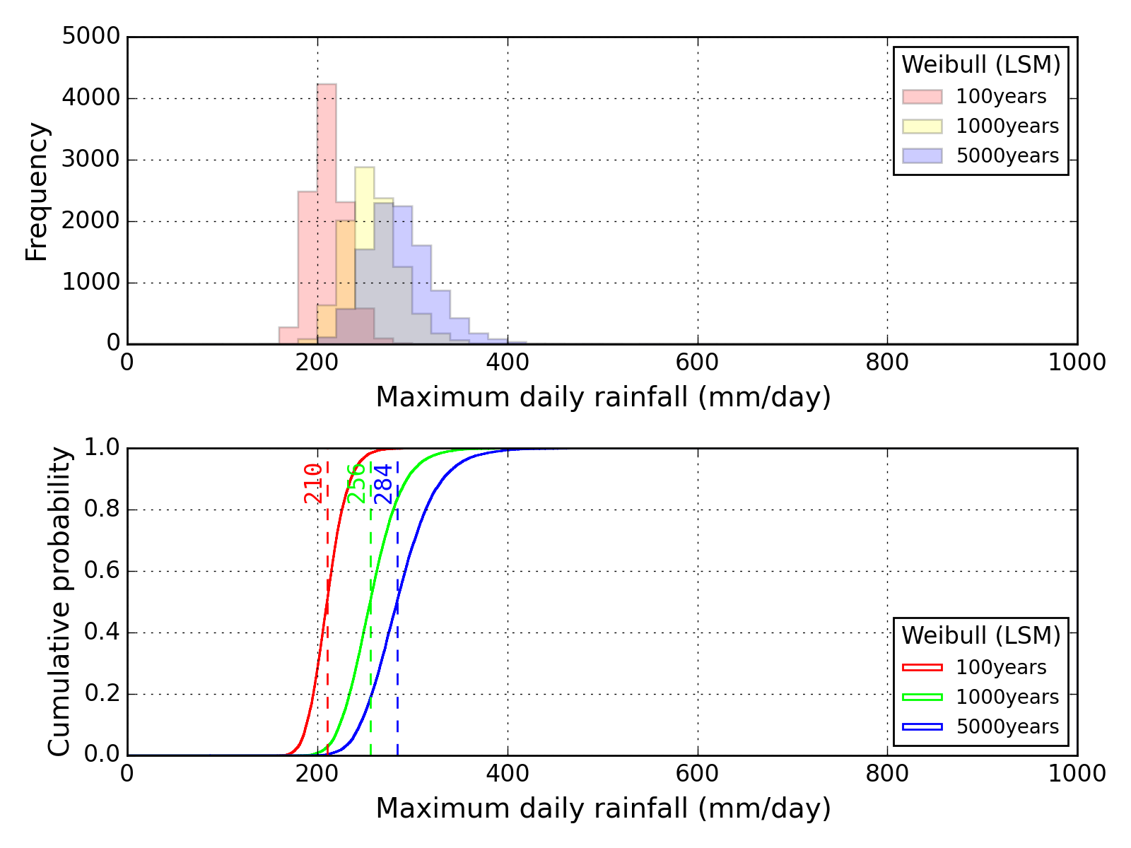
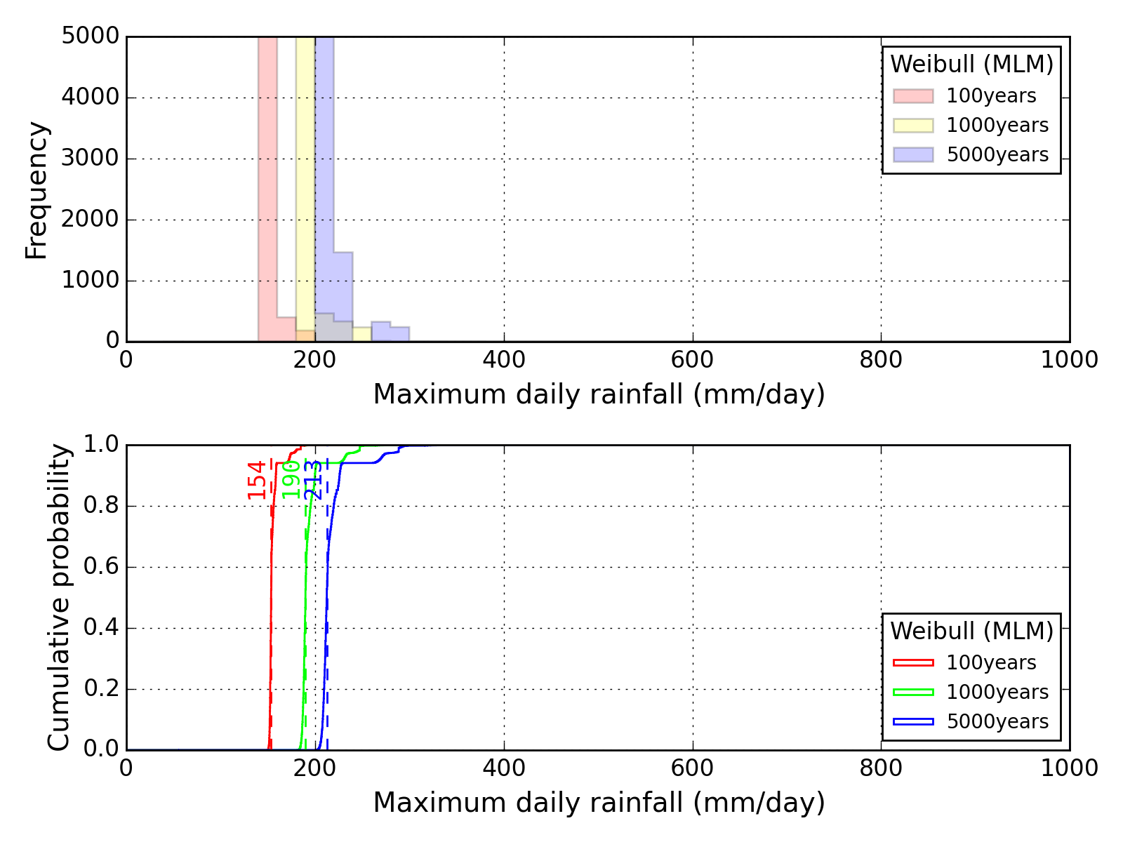
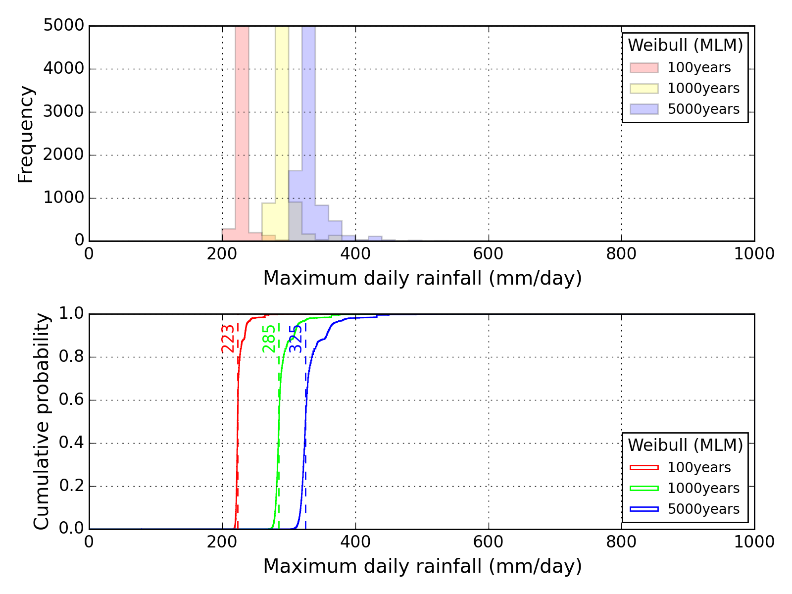
Statistical estimation by Bootstrap method
The method to obtain the point estimate and confidence interval by Bootstrap method is shown in this section.
The procedure by Bootstrap method is shown below.
Rejection Test
In usual, the very large or small value which seem to be singular in an ordinary sense are to be contained in hydrologic observations.
In hydrologic frequency analysis, the rejection test is carried out in order to decide adoption or rejection of the singular variant.
In this section, the procedure of rejection test for the singular variant is introduced.
- [Subject] Carry out the rejection test for maximim value $x_{\epsilon}$ which is contained in a sample with size of $N$ .
(The maximum value $x_{\epsilon}$ is the targeted value of the rejection test.)
- (1) Calculate the limit singular level $\epsilon_0$ for the significant level $\beta_0$ using following equation:
\begin{equation}
\epsilon_0=1-(1-\beta_0)^{1/N} \qquad \text{(normally, $\beta_0$=5\%)}
\end{equation}
- (2) Select the type of probability distribution model and estimate parameters using the dataset with sample size of $N-1$ except the targeted value $x_{\epsilon}$ which is seemed singular value.
- (3) Estimate the exceedance probability $p$ for targeted value $x_{\epsilon}$ using adopted provability distribution model.
- (4) Estimate the \% point of the standard mormal distribution $u_{\epsilon}$, which has equal exceedance probability $p$ for targeted value $x_{\epsilon}$ on adopted probability distribution model.
It means to get the value of $u_{\epsilon}$ satisfied following condition.
Where, $\Phi$ is the cumulative distribution function of standard normal distribution and $F$ is the cumulative distribution function adopted for observed sample.
\begin{equation}
\text{Exceedance probability}\quad p=1-F(x_{\epsilon})=1-\Phi(u_{\epsilon})
\end{equation}
- (5) If the targeted value belongs to the population to which the sample with size of $N-1$ except targeted value belongs,
F-value expressed below shall follow the F-distribution with the degrees of freedom of $(1,M-1)$ .
Note that $M(=N-1)$ means sample size except the targeted value.
\begin{equation}
F=\left(\frac{M-1}{M+1}\right)\cdot u_{\epsilon}{}^2
\end{equation}
So, calculate the probability on F-distribution $2\epsilon$ which satisfies following condition:
\begin{equation}
F_{M-1}^1 (2\epsilon)=\left(\frac{M-1}{M+1}\right)\cdot u_{\epsilon}{}^2
\end{equation}
- (6) Decide adoption or rejection by comparison between $\epsilon$ defined by targeted value and $\epsilon_0$ defined by specified significant level $\beta_0$ .
The detailed craiteria is shown below:
\begin{equation}
\begin{cases}
\epsilon \leqq \epsilon_0 &\text{The exceedance probability for the targeted value is smaller than or equal to}\\
&\text{limit singular level.}\\
&\text{Therefore, the targeted value shall be rejected. (don't use it in the analysis)}\\
\epsilon > \epsilon_0 &\text{The exceedance provability for the targeted value is larger than limit singular level.}\\
&\text{Therefore, the targeted value cannot be rejected. (use it in the analysis)}
\end{cases}
\end{equation}
(Notice) Applying method for the probability distributions except normal
Rejection test method using F-distribution is based of the theorem for only normal distribution.
Therefore, steps (2)(3)(4) are adopted in order to treat all probability distribution models.
In shown above, it is possible to treat all probability distribution models by using the \% point of standard normal distribution which has the same exceedance probability for targeted value on selected probability distribution model.
References
- http://thesis.ceri.go.jp/center/info/geppou/ceri/0005005050.html
(Hoshi Kiyoshi, Monthly report of Civil Engineering Research Institute, No.540, May 1998)
- http://iss.ndl.go.jp/books/R000000004-I4497918-00
(Hoshi Kiyoshi, Monthly report of Civil Engineering Research Institute, No.540, May 1998)
- http://iss.ndl.go.jp/books/R000000004-I4522177-00
(Hoshi Kiyoshi, Shinme Ryuichi, Miyahara Masayuki, Monthly report of Civil Engineering Research Institute, No.541 June 1998)
- Yoshimi GODA, Masanobu KUDAKA and Hiroyasu KAWAI : Use of L-moments Method for Extreme Statistics of Storm Wave Height, Vol.B2-65, No.1, 2009, 161-165, Journal of JSCE
- Derek A. Roff, ISBN978-4-320-05714-2 (Introduction to Computer-Intensive Methods of data Analysis in Biology, translated by Nomakuchi Shintaro into japanese)
- Mutsumi KADOYA : Application of Extreme Value Distribution in Hydrologic Frequency Analysis Part II. Singular Hydrologic Amount and Rejection Test, Citation Bulletins - Disaster Prevention Research Institute, Kyoto University (1964), 66: 33-44, 1964-03-25 (URL http://hdl.handle.net/2433/123738)
Programs
Program 'f90_qq.f90' and 'f90_bts.f90' can treat following probability distribution models.
| No | Short form | Probability distribution function | Parameters |
|---|
| 1 | Gumbel | Gumbel distribution | 2 |
| 2 | GEV | Generalized Extreme Value distribution | 3 |
| 3 | Weibull (Goda) | Weibull distribution (L-moments by Goda) | 3 |
| 4 | Weibull (LSM) | Weibull distribution (Least Square Method) | 3 |
| 5 | Weibull (MLM) | Weibull distribution (Maximum Likelihood Method) | 3 |
| 6 | SQRT-ET | SQRT exponential-type distribution of maximum | 2 |
| 7 | LP3 | Log Pearson type III distribution | 3 |
| 8 | LN3 (Iwai) | Logarithmic Normal distribution (Iwai method: quantile) | 3 |
| 9 | LN3 (Moment) | Logarithmic Normal distribution (Moment method) | 3 |
| 10 | LN3 (Trial) | Logarithmic Normal distribution (Trial method) | 3 |
| 11 | Exponential | Exponential distribution | 2 |
| 12 | GPD | Generalized Pareto distribution | 3 |
Quantile
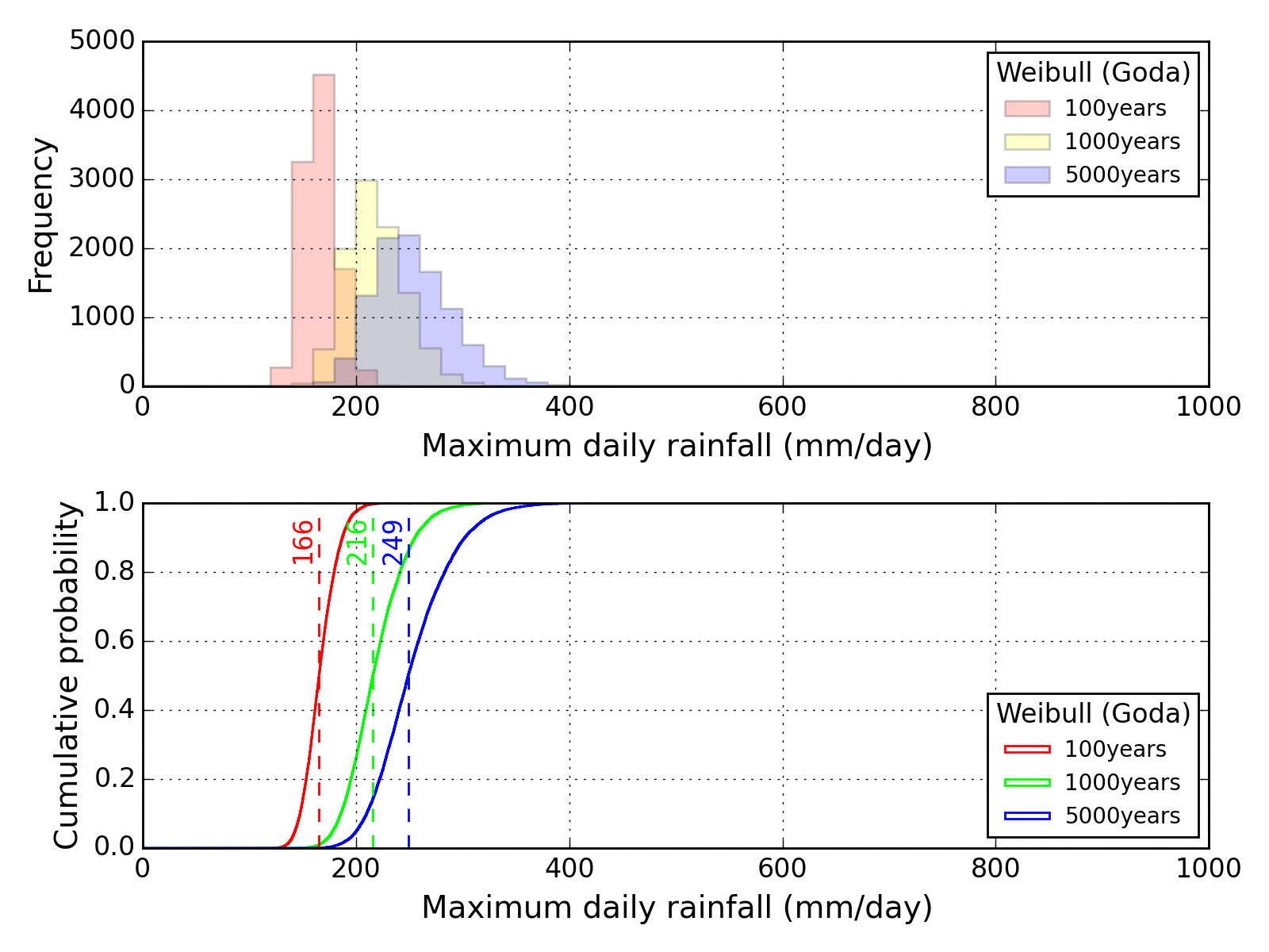
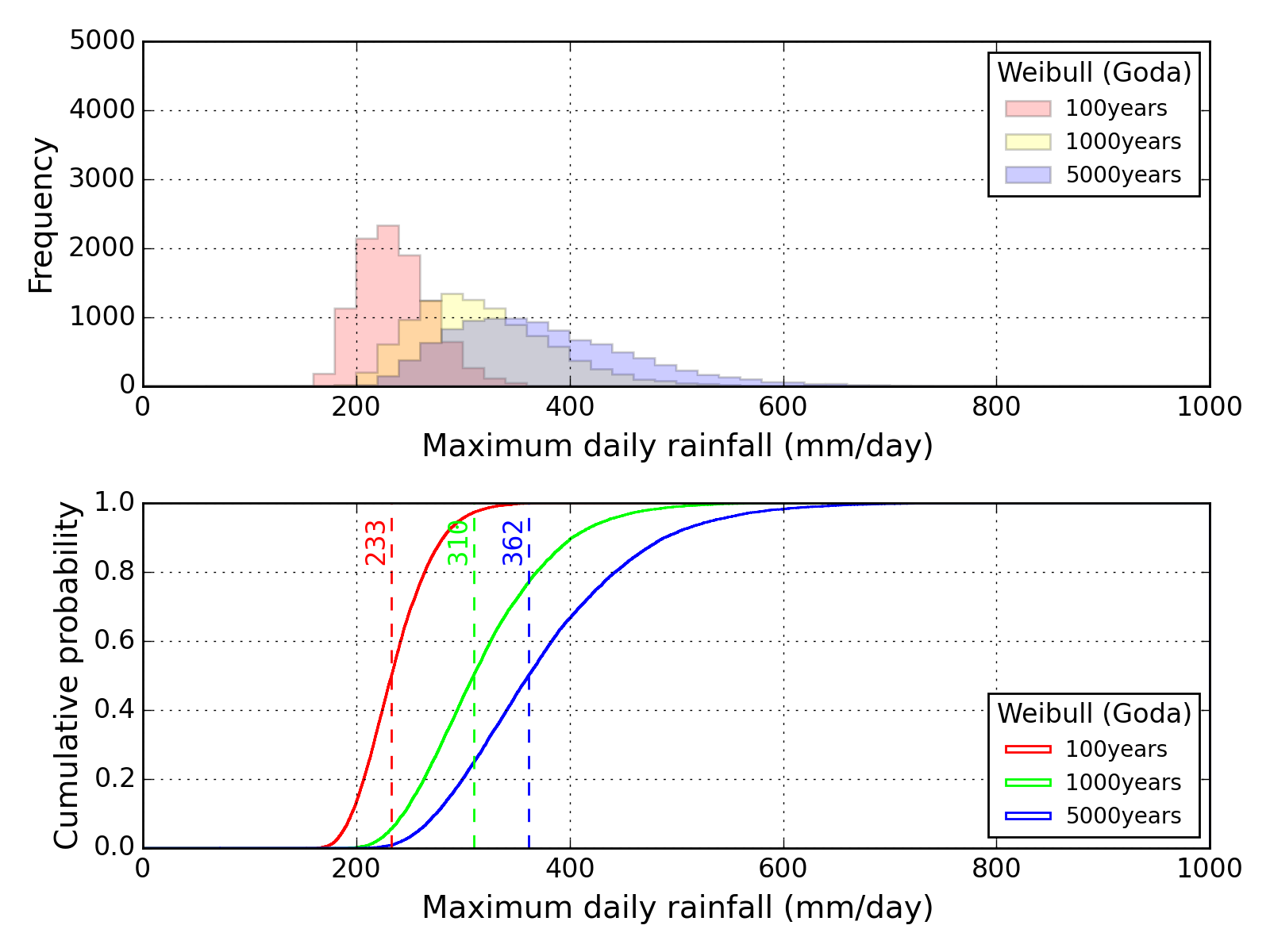
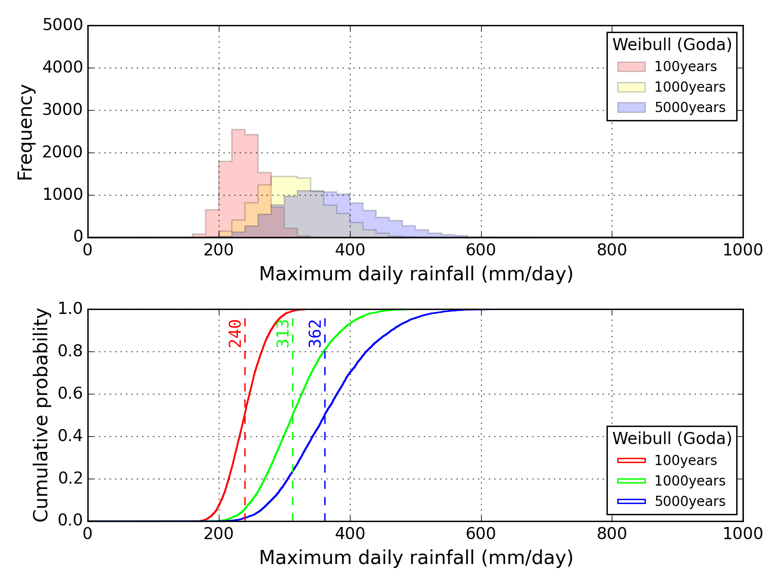
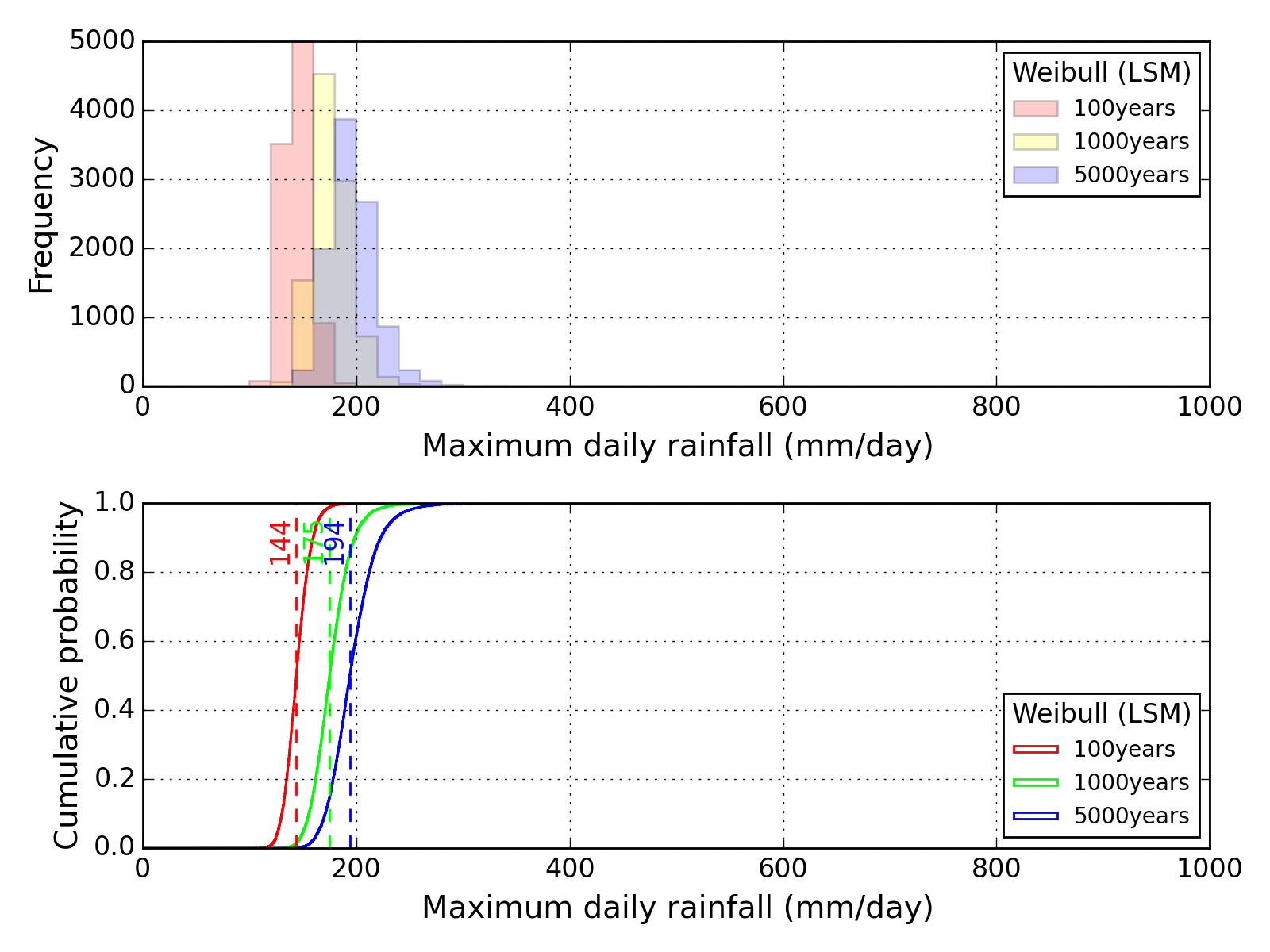
Bootstrap
Output samples
Results of parameter estimation
| Sappro |
|---|
| No | Model | Parameters | r |
|---|
| 1 | GUM | (*_a_b) | ------ | 23.2287 | 54.6021 | 0.9910 |
| 2 | GEV | (k_a_b) | -0.1204 | 20.5086 | 53.3511 | 0.9953 |
| 3 | WGO | (k_a_c) | 1.2653 | 41.0969 | 29.8365 | 0.9943 |
| 4 | WLS | (k_a_c) | 1.8362 | 53.5212 | 20.0000 | 0.9818 |
| 5 | WML | (k_a_c) | 1.6878 | 54.0180 | 20.0000 | 0.9859 |
| 6 | SQR | (a_b_*) | 62.1595 | 0.6967 | ------ | 0.9953 |
| 7 | LP3 | (a_b_c) | 0.0491 | 70.8151 | 0.6545 | 0.9958 |
| 8 | LNQ | (a_m_s) | 11.8395 | 3.8956 | 0.5190 | 0.9959 |
| 9 | LNM | (a_m_s) | 1.6808 | 4.0990 | 0.4372 | 0.9949 |
| 10 | LNT | (a_m_s) | 8.2000 | 3.9740 | 0.4875 | 0.9958 |
| 11 | EXP | (*_a_c) | ------ | 32.2018 | 35.8079 | 0.9911 |
| 12 | GPD | (k_a_c) | 0.2019 | 42.6095 | 32.5574 | 0.9905 |
| Maebashi |
|---|
| No | Model | Parameters | r |
|---|
| 1 | GUM | (*_a_b) | ------ | 30.6850 | 78.4176 | 0.9587 |
| 2 | GEV | (k_a_b) | -0.1811 | 25.1676 | 76.0772 | 0.9887 |
| 3 | WGO | (k_a_c) | 1.1211 | 48.0942 | 50.0044 | 0.9721 |
| 4 | WLS | (k_a_c) | 1.5103 | 59.8866 | 41.3000 | 0.9528 |
| 5 | WML | (k_a_c) | 1.3833 | 60.3496 | 41.3000 | 0.9593 |
| 6 | SQR | (a_b_*) | 124.5701 | 0.6175 | ------ | 0.9799 |
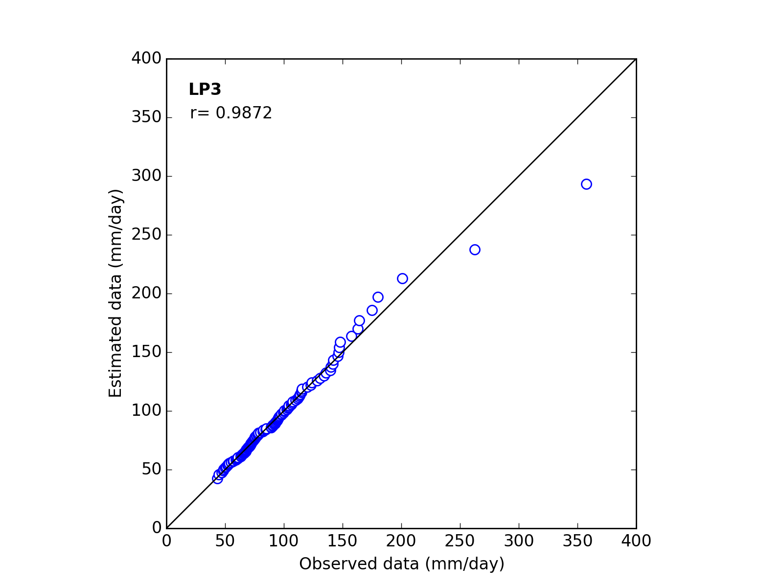
| 7 | LP3 | (a_b_c) | 0.1244 | 9.2123 | 3.3424 | 0.9872 |
| 8 | LNQ | (a_m_s) | 34.7338 | 3.9124 | 0.6483 | 0.9860 |
| 9 | LNM | (a_m_s) | 37.0289 | 3.8600 | 0.6622 | 0.9866 |
| 10 | LNT | (a_m_s) | 30.0000 | 4.0187 | 0.5909 | 0.9830 |
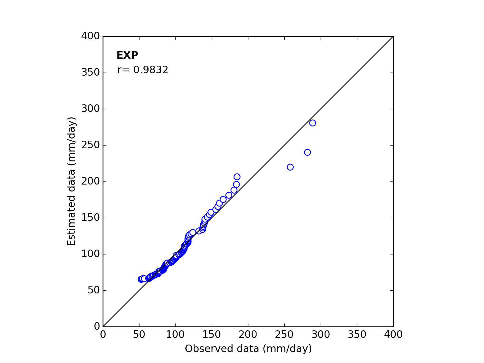
| 11 | EXP | (*_a_c) | ------ | 42.5384 | 53.5906 | 0.9768 |
| 12 | GPD | (k_a_c) | 0.0979 | 48.9890 | 51.5083 | 0.9664 |
| Kyoto |
|---|
| No | Model | Parameters | r |
|---|
| 1 | GUM | (*_a_b) | ------ | 29.9941 | 89.3022 | 0.9710 |
| 2 | GEV | (k_a_b) | -0.1593 | 25.2824 | 87.2494 | 0.9883 |
| 3 | WGO | (k_a_c) | 1.1704 | 49.1276 | 60.0933 | 0.9797 |
| 4 | WLS | (k_a_c) | 1.6323 | 63.0903 | 49.5000 | 0.9618 |
| 5 | WML | (k_a_c) | 1.4936 | 63.5526 | 49.5000 | 0.9676 |
| 6 | SQR | (a_b_*) | 259.3959 | 0.6786 | ------ | 0.9849 |
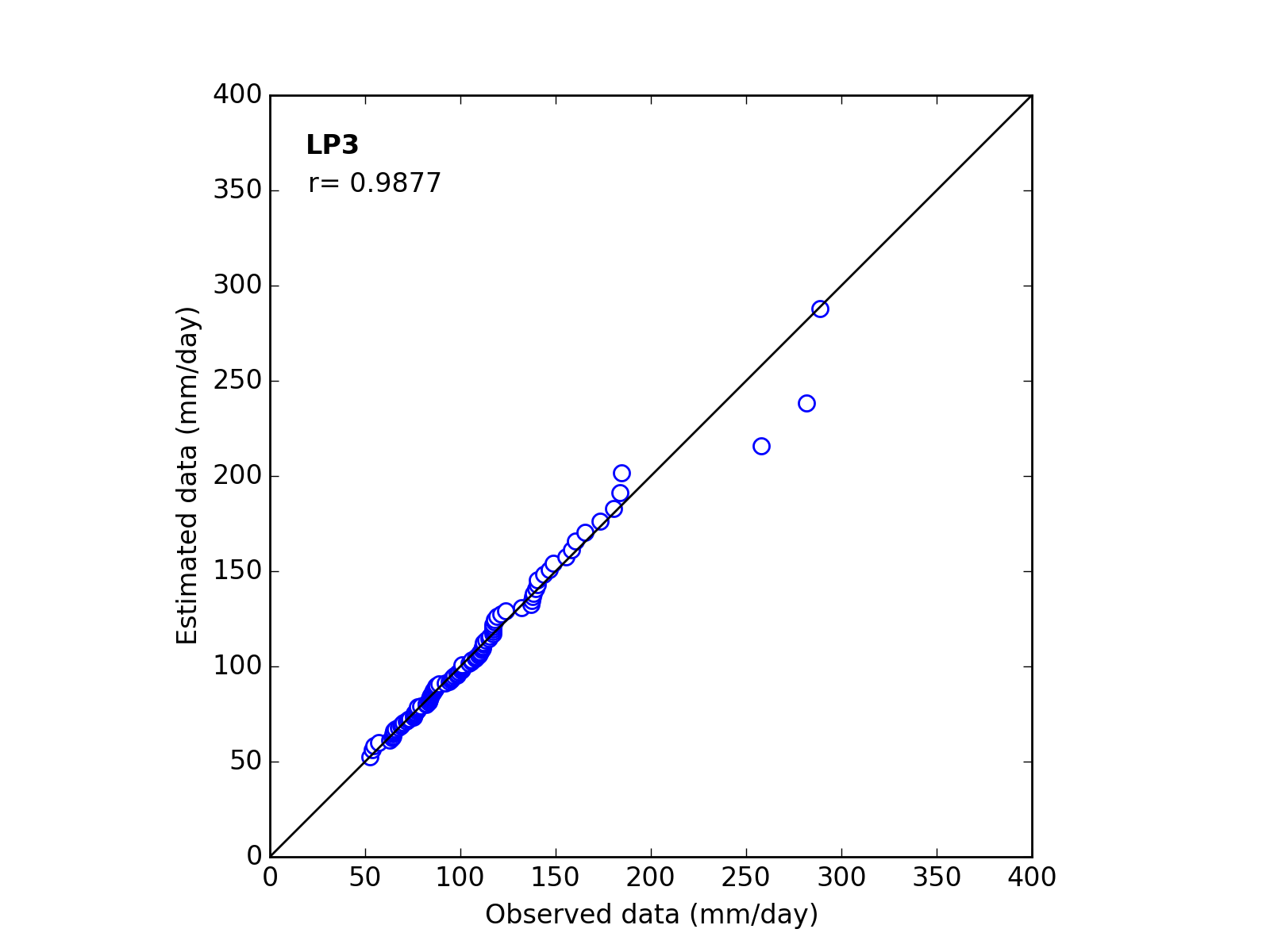
| 7 | LP3 | (a_b_c) | 0.1140 | 8.6225 | 3.6260 | 0.9877 |
| 8 | LNQ | (a_m_s) | 37.4759 | 4.0874 | 0.5426 | 0.9855 |
| 9 | LNM | (a_m_s) | 38.5954 | 4.0606 | 0.5642 | 0.9864 |
| 10 | LNT | (a_m_s) | 36.5000 | 4.1043 | 0.5433 | 0.9856 |
| 11 | EXP | (*_a_c) | ------ | 41.5806 | 65.0342 | 0.9832 |
| 12 | GPD | (k_a_c) | 0.1348 | 50.3628 | 62.2327 | 0.9743 |
Q-Q plot
| Sapporo | Maebashi | Kyoto |
|---|
 |
 |
 |
 |
 |
 |
 |
 |
 |
 |
 |
 |
 |
 |
 |
 |
 |
 |
 |
 |
 |
 |
 |
 |
 |
 |
 |
 |
 |
 |
 |
 |
 |
 |
 |
 |
| Sapporo | Maebashi | Kyoto |
|---|
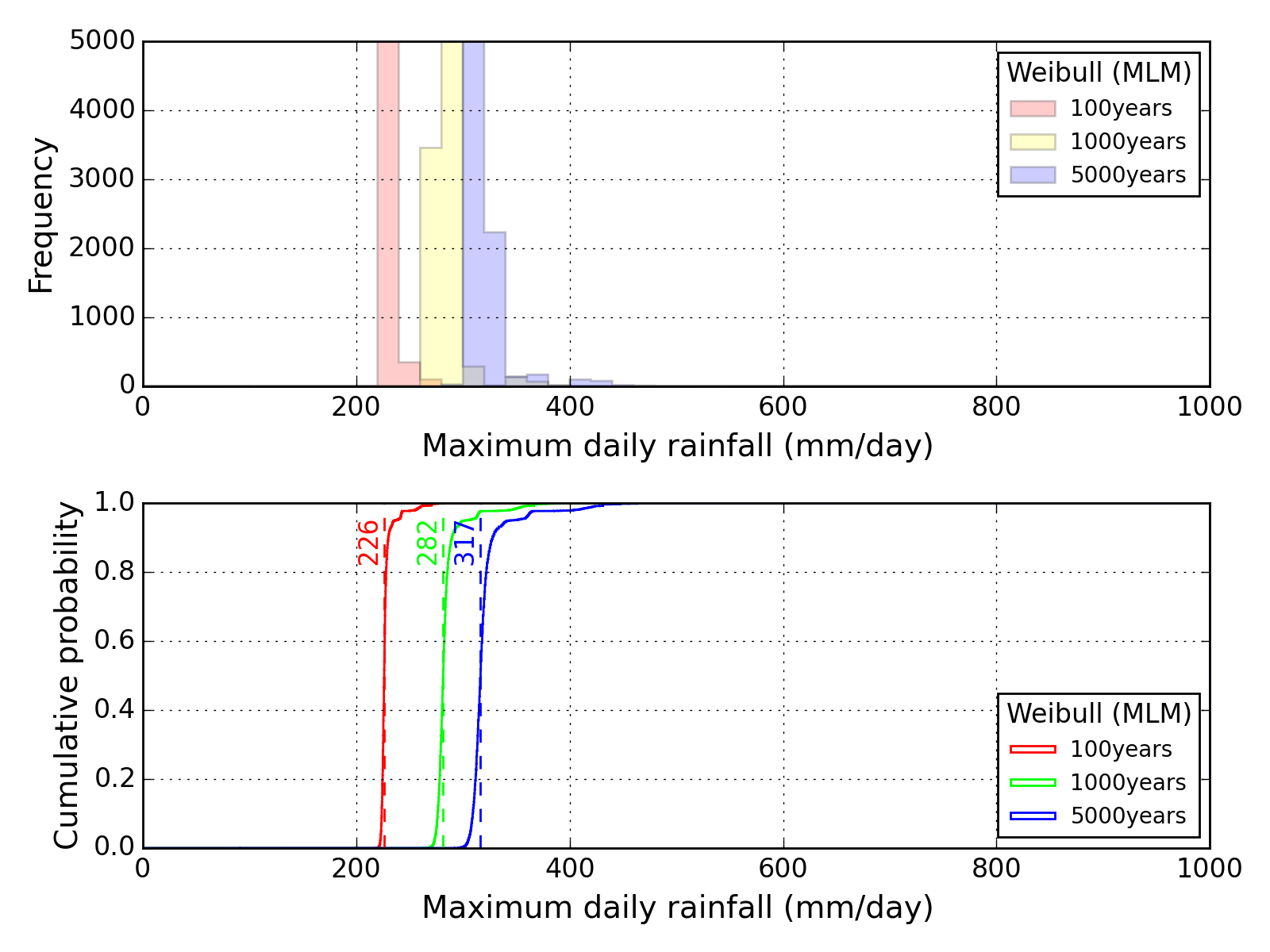
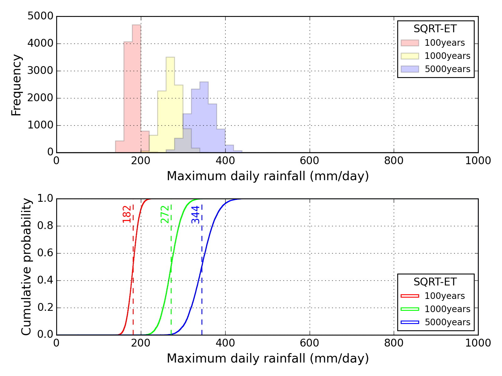
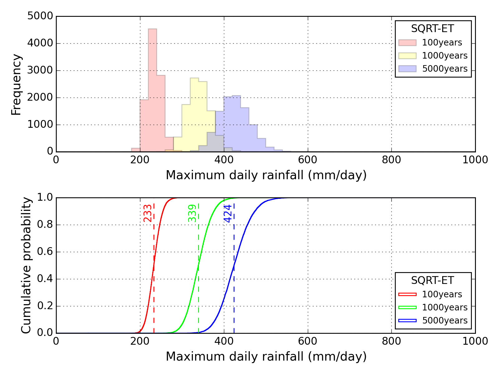
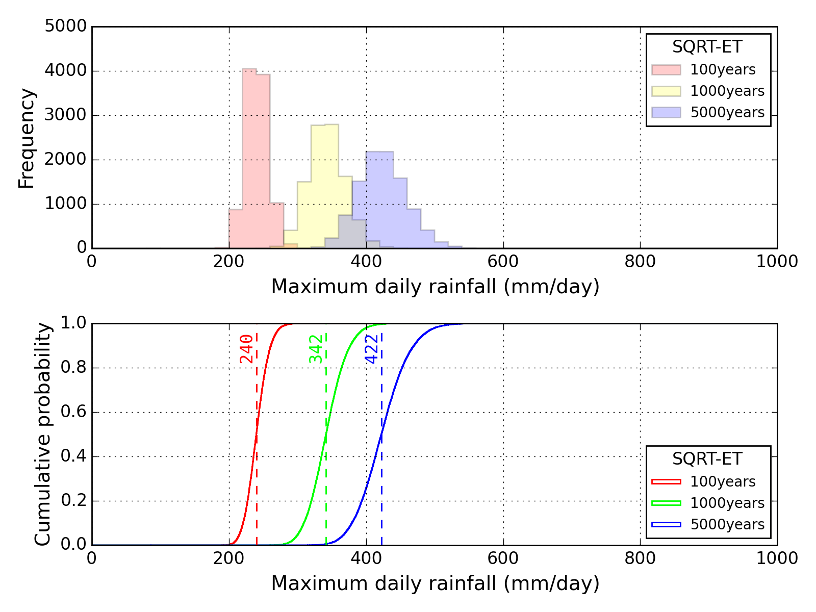
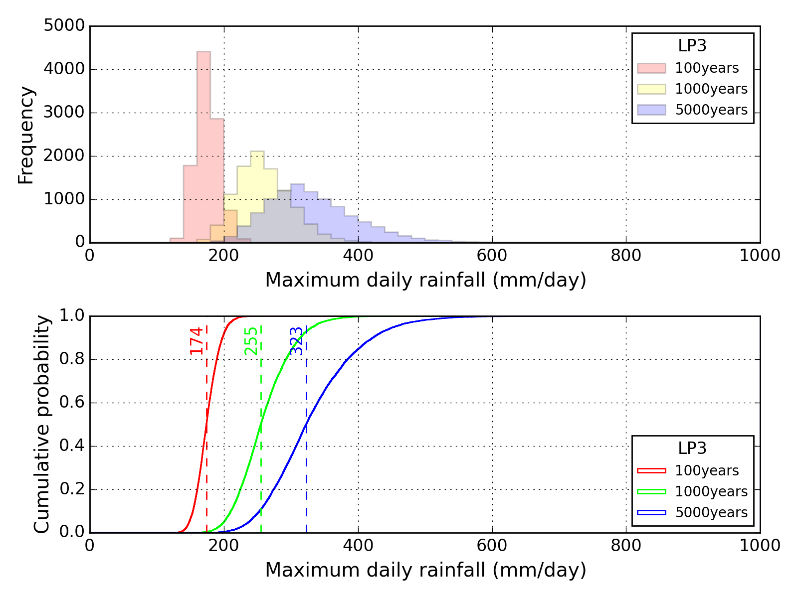
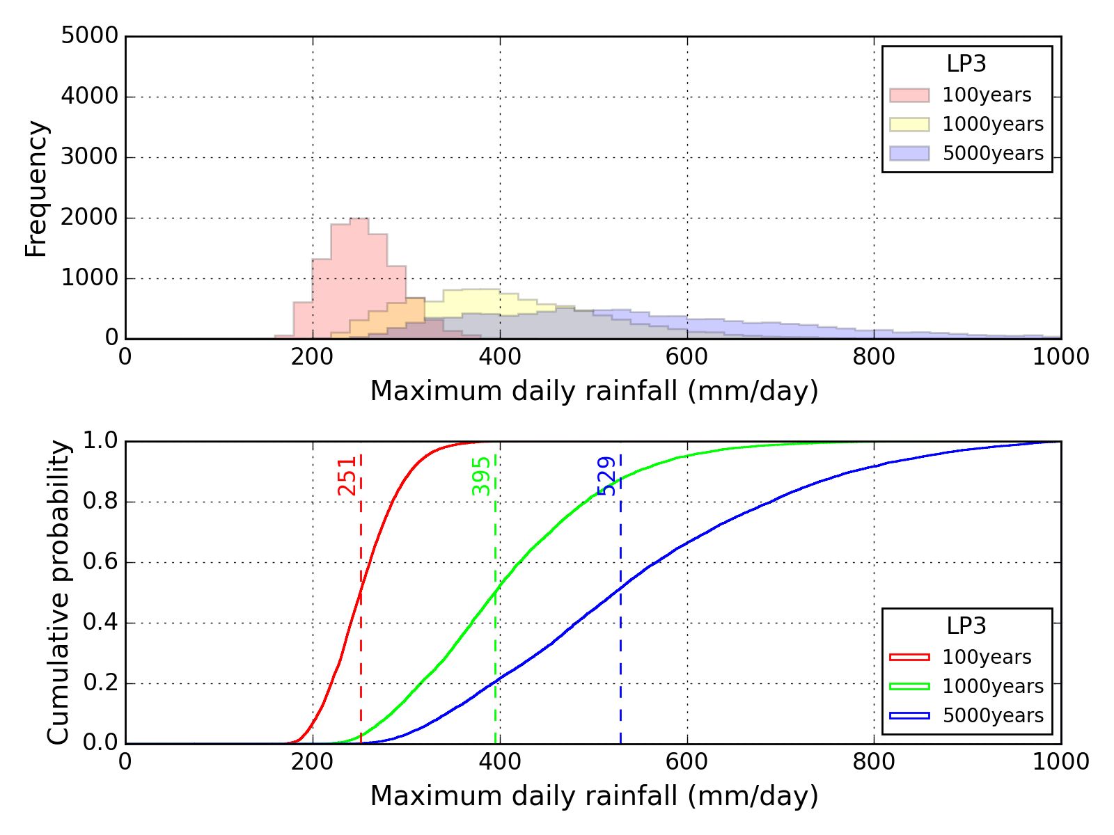
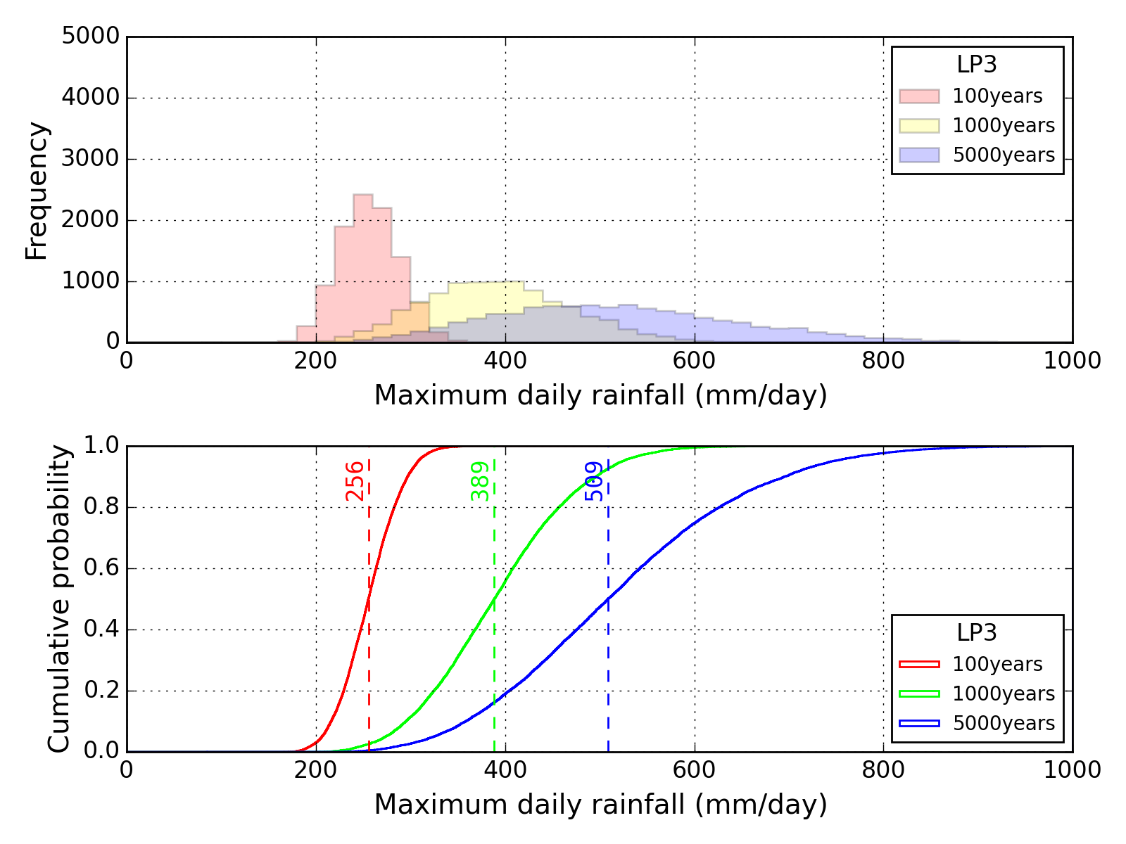
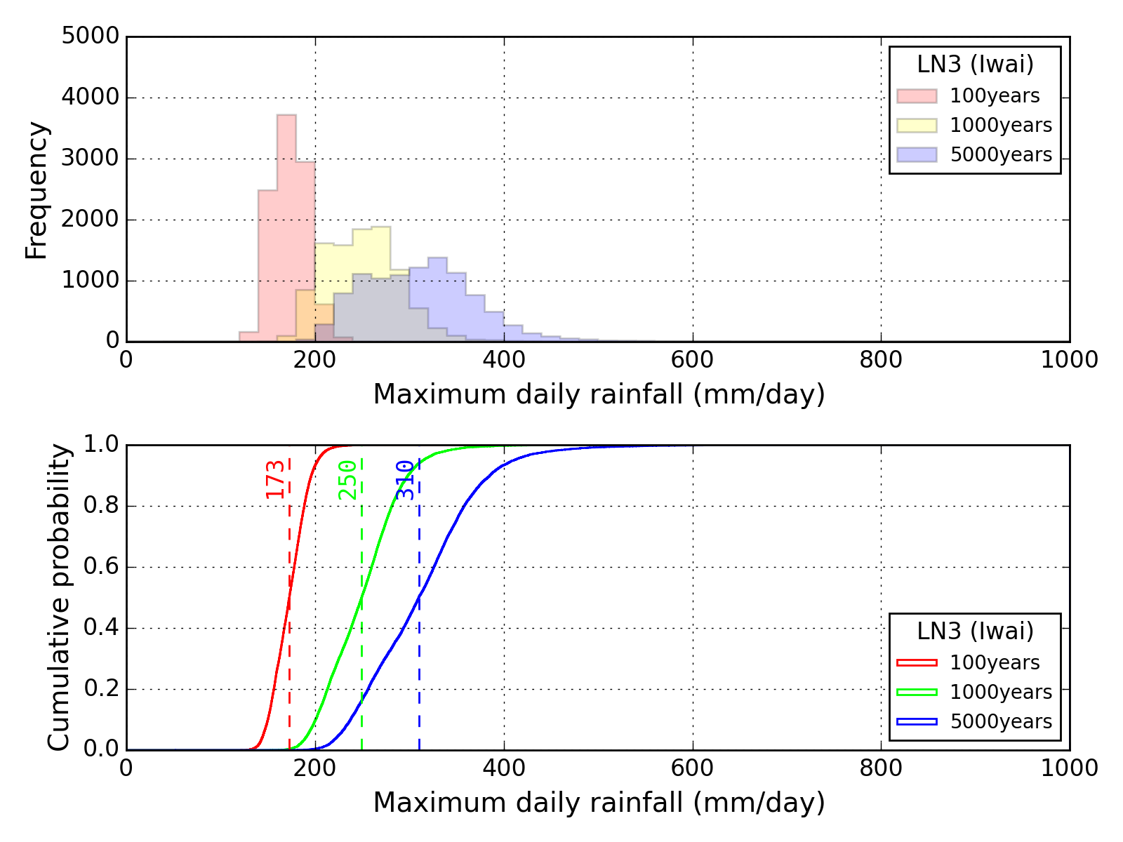
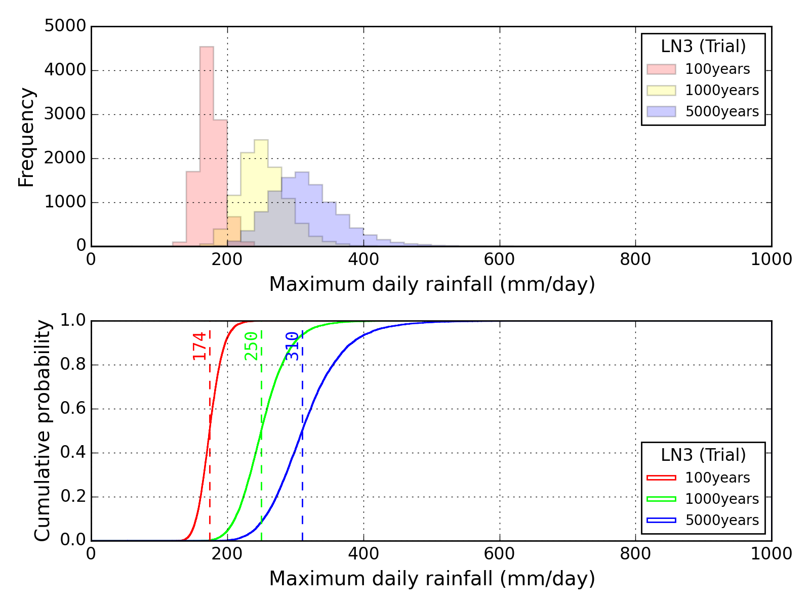
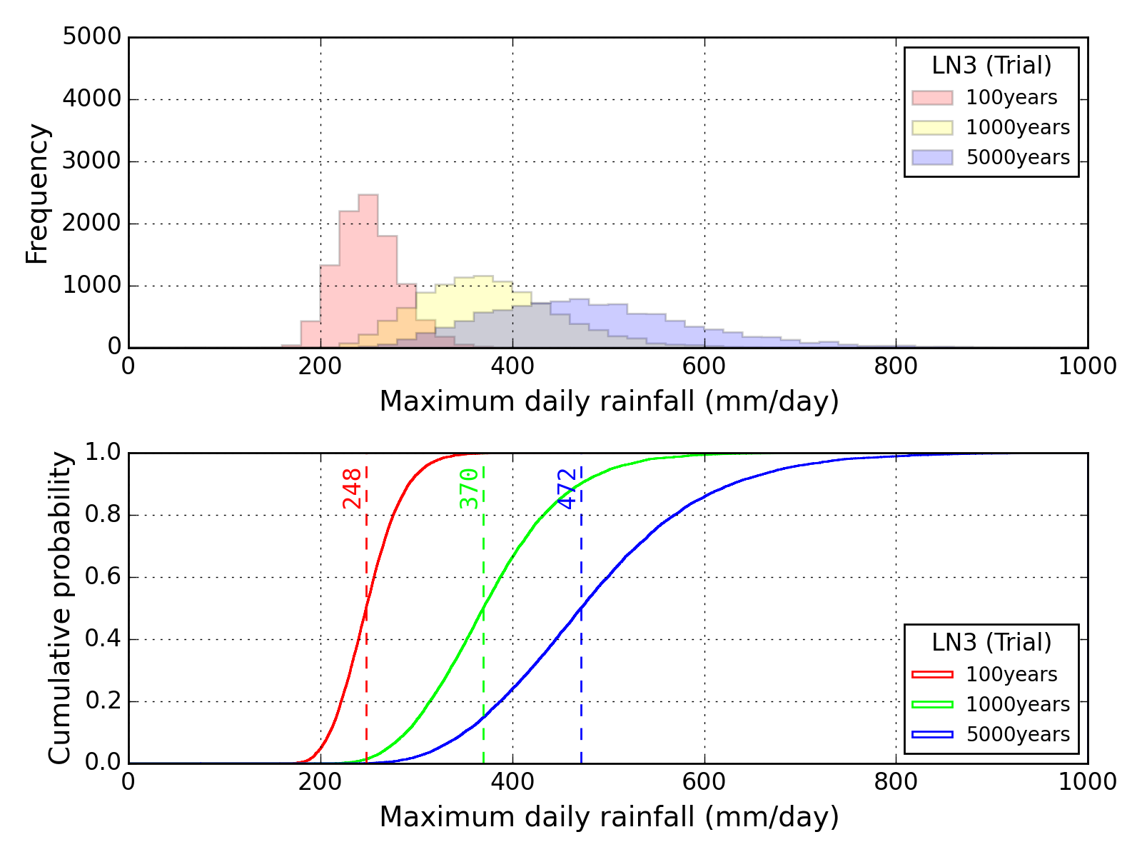
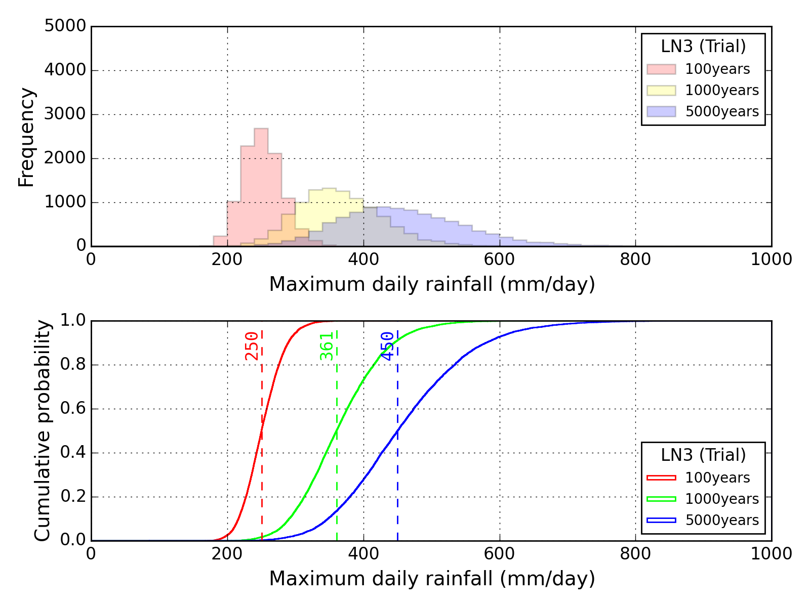
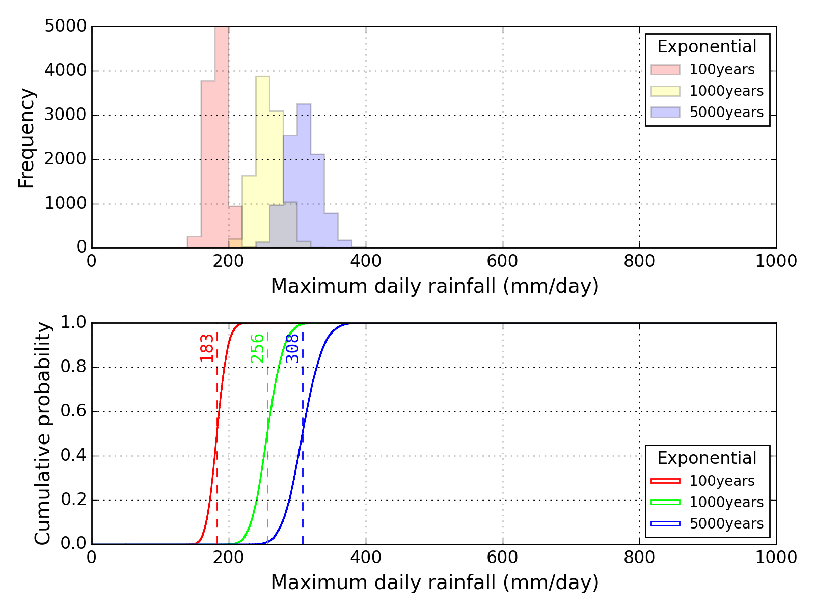
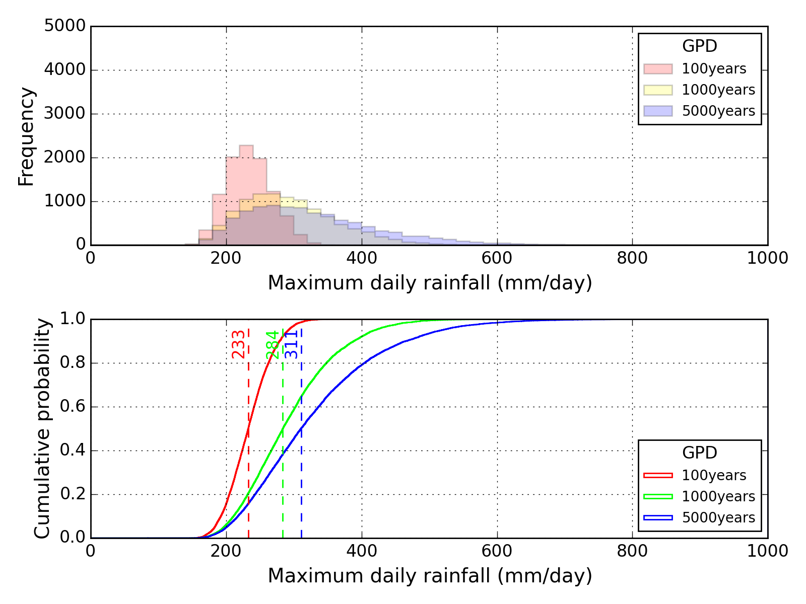
Bootstrap method
| Sapporo | Maebashi | Kyoto |
|---|
 |
 |
 |
 |
 |
 |
 |
 |
 |
 |
 |
 |
 |
 |
 |
 |
 |
 |
 |
 |
 |
 |
 |
 |
 |
 |
 |
 |
 |
 |
 |
 |
 |
 |
 |
 |
| Sapporo | Maebashi | Kyoto |
|---|