Contents
Equation of Motion of SDOF
The equation of motion of SDOF system at instance $t+\Delta t$ is shown below, where dot means differentiation by time $t$ .
\begin{equation}
m\cdot\ddot{u}(t+\Delta t)+c\cdot\dot{u}(t+\Delta t)+k\cdot u(t+\Delta t)=f(t+\Delta t)
\end{equation}
| where, | $m$ | : mass | | $\ddot{u}$ | : acceleration | | $f$ | : external force |
| | $c$ | : damping | | $\dot{u}$ | : velocity | | | |
| | $k$ | : stiffness | | $u$ | : displacement | | | |
Solution of equation of motion: Linear acceleration method
Displacement
Use Taylor series for the displacement $u$ at $t+\Delta t$ and consider the terms from 1st to 4th of the right side.
\begin{align}
u(t+\Delta t)&=u(t)+\frac{\Delta t}{1!}\cdot\dot{u}(t)+\frac{(\Delta t)^2}{2!}\cdot\ddot{u}(t)+\frac{(\Delta t)^3}{3!}\cdot\dddot{u}(t)+\cdots \\
&=u(t)+\Delta t\cdot\dot{u}(t)+\frac{(\Delta t)^2}{3}\cdot\ddot{u}(t)+\frac{(\Delta t)^2}{6}\cdot\ddot{u}(t+\Delta t)
\end{align}
In the linear acceleration method, the differential coefficient of 3rd order of the displacement $u$ is linearized using following equation.
\begin{equation}
\dddot{u}(t)=\frac{\ddot{u}(t+\Delta t)-\ddot{u}(t)}{\Delta t}
\end{equation}
Velocity
Using a trapezoidal formula, following form can be obtained.
\begin{equation}
\dot{u}(t+\Delta t)=\dot{u}(t)+\int_t^{t+\Delta t}\ddot{u}(t)dt
=\dot{u}(t)+\frac{\Delta t}{2}\cdot\left(\ddot{u}(t+\Delta t)+\ddot{u}(t)\right)
\end{equation}
Acceleration
Substituting the displacement and velocity which are derived from above to the equation of motion, following form to calculate the acceleration can be obtained.
\begin{equation}
\ddot{u}(t+\Delta t)=
\cfrac{f(t+\Delta t)-c\cdot\left(\dot{u}(t)+\cfrac{\Delta t}{2}\cdot\ddot{u}(t)\right)-k\cdot\left(u(t)+\Delta t\cdot\dot{u}(t)+\cfrac{(\Delta t)^2}{3}\cdot\ddot{u}(t)\right)}
{m+c\cdot\cfrac{\Delta t}{2}+k\cdot\cfrac{(\Delta t)^2}{6}}
\end{equation}
Summary
Linear Acceleration Method
\begin{align}
\ddot{u}(t+\Delta t)=&
\cfrac{f(t+\Delta t)-c\cdot\left(\dot{u}(t)+\cfrac{\Delta t}{2}\cdot\ddot{u}(t)\right)-k\cdot\left(u(t)+\Delta t\cdot\dot{u}(t)+\cfrac{(\Delta t)^2}{3}\cdot\ddot{u}(t)\right)}
{m+c\cdot\cfrac{\Delta t}{2}+k\cdot\cfrac{(\Delta t)^2}{6}}\\
\dot{u}(t+\Delta t)=&
\dot{u}(t)+\frac{\Delta t}{2}\cdot\ddot{u}(t)+\frac{\Delta t}{2}\cdot\ddot{u}(t+\Delta t)\\
u(t+\Delta t)=&
u(t)+\Delta t\cdot\dot{u}(t)+\frac{(\Delta t)^2}{3}\cdot\ddot{u}(t)+\frac{(\Delta t)^2}{6}\cdot\ddot{u}(t+\Delta t)
\end{align}
Solution of equation of motion: Average acceleration method
Displacement
Use Taylor series for the displacement $u$ at $t+\Delta t$ and consider the terms from 1st to 3rd of the right side.
\begin{align}
u(t+\Delta t)&=u(t)+\frac{\Delta t}{1!}\cdot\dot{u}(t)+\frac{(\Delta t)^2}{2!}\cdot\ddot{u}(t)+\cdots \\
&=u(t)+\Delta t\cdot\dot{u}(t)+\frac{(\Delta t)^2}{4}\cdot\ddot{u}(t)+\frac{(\Delta t)^2}{4}\cdot\ddot{u}(t+\Delta t)
\end{align}
In the average acceleration method, the differential coefficient of 2nd order of the displacement $u$ is linearized using following equation.
\begin{equation}
\ddot{u}(t)=\frac{\ddot{u}(t+\Delta t)+\ddot{u}(t)}{2}
\end{equation}
Velocity
Similar to the case of the linear acceleration method, following equation can be obtained.
\begin{equation}
\dot{u}(t+\Delta t)=\dot{u}(t)+\int_t^{t+\Delta t}\ddot{u}(t)dt
=\dot{u}(t)+\frac{\Delta t}{2}\cdot\left(\ddot{u}(t+\Delta t)+\ddot{u}(t)\right)
\end{equation}
Acceleration
Substituting the displacement and velocity which are derived from above to the equation of motion, following form to calculate the acceleration can be obtained.
\begin{equation}
\ddot{u}(t+\Delta t)=
\cfrac{f(t+\Delta t)-c\cdot\left(\dot{u}(t)+\cfrac{\Delta t}{2}\cdot\ddot{u}(t)\right)-k\cdot\left(u(t)+\Delta t\cdot\dot{u}(t)+\cfrac{(\Delta t)^2}{4}\cdot\ddot{u}(t)\right)}
{m+c\cdot\cfrac{\Delta t}{2}+k\cdot\cfrac{(\Delta t)^2}{4}}
\end{equation}
Summary
Average Acceleration method
\begin{align}
\ddot{u}(t+\Delta t)=&
\cfrac{f(t+\Delta t)-c\cdot\left(\dot{u}(t)+\cfrac{\Delta t}{2}\cdot\ddot{u}(t)\right)-k\cdot\left(u(t)+\Delta t\cdot\dot{u}(t)+\cfrac{(\Delta t)^2}{4}\cdot\ddot{u}(t)\right)}
{m+c\cdot\cfrac{\Delta t}{2}+k\cdot\cfrac{(\Delta t)^2}{4}}\\
\dot{u}(t+\Delta t)=&
\dot{u}(t)+\frac{\Delta t}{2}\cdot\ddot{u}(t)+\frac{\Delta t}{2}\cdot\ddot{u}(t+\Delta t)\\
u(t+\Delta t)=&
u(t)+\Delta t\cdot\dot{u}(t)+\frac{(\Delta t)^2}{4}\cdot\ddot{u}(t)+\frac{(\Delta t)^2}{4}\cdot\ddot{u}(t+\Delta t)
\end{align}
Solution of equation of motion: Nermark's β method
Formula for calculation
This method is a generalized method of the linear acceleration method. The use of Taylor series for the displacement $u$ and velocity $\dot{u}$ at $t+\Delta t$ provides following forms.
\begin{align}
u(t+\Delta t)&=u(t)+\frac{\Delta t}{1!}\cdot\dot{u}(t)+\frac{(\Delta t)^2}{2!}\cdot\ddot{u}(t)+\frac{(\Delta t)^3}{3!}\cdot\dddot{u}(t)+\cdots \\
\dot{u}(t+\Delta t)&=\dot{u}(t)+\frac{\Delta t}{1!}\cdot\ddot{u}(t)+\frac{(\Delta t)^2}{2!}\cdot\dddot{u}(t)+\cdots
\end{align}
If we deem the 4th term for displacement as $\beta=1/3!$ , the 3rd term for velocity as $\gamma=1/2!$ , and we truncate higher order terms, above equation are expressed as follows.
\begin{align}
u(t+\Delta t)&=u(t)+\Delta t\cdot\dot{u}(t)+\frac{(\Delta t)^2}{2}\cdot\ddot{u}(t)+\beta\cdot(\Delta t)^3\cdot\dddot{u}(t) \\
\dot{u}(t+\Delta t)&=\dot{u}(t)+\Delta t\cdot\ddot{u}(t)+\gamma\cdot(\Delta t)^2\cdot\dddot{u}(t)
\end{align}
Next, similar to the linear acceleration method, we liniearize the term of $\dddot{u}$ as follow.
\begin{equation}
\dddot{u}(t)=\frac{\ddot{u}(t+\Delta t)-\ddot{u}(t)}{\Delta t}
\end{equation}
To arrange the equation of motion using above relationship provides following equations.
\begin{align}
u(t+\Delta t)&=u(t)+\Delta t\cdot\dot{u}(t)+\left(\frac{1}{2}-\beta\right)(\Delta t)^2\cdot\ddot{u}(t)+\beta(\Delta t)^2\cdot\ddot{u}(t+\Delta t) \\
\dot{u}(t+\Delta t)&=\dot{u}(t)+(1-\gamma)\cdot\Delta t\cdot\ddot{u}(t)+\gamma\cdot\Delta t\cdot\ddot{u}(t+\Delta t)
\end{align}
The formulas for Newmark's β method can be expressed as follow by taking into consideration of $\gamma=1/2$ . (Regarding the value of $\gamma$ , $\gamma=1/2$ is normally used because of stability of solution)
Newmark's β method
\begin{align}
\ddot{u}(t+\Delta t)=&
\cfrac{f(t+\Delta t)-c\cdot\left(\dot{u}(t)+\cfrac{\Delta t}{2}\cdot\ddot{u}(t)\right)-k\cdot\left(u(t)+\Delta t\cdot\dot{u}(t)+\left(\cfrac{1}{2}-\beta\right)\cdot(\Delta t)^2\cdot\ddot{u}(t)\right)}
{m+c\cdot\cfrac{\Delta t}{2}+k\cdot\beta\cdot(\Delta t)^2}\\
\dot{u}(t+\Delta t)=&
\dot{u}(t)+\frac{\Delta t}{2}\cdot\ddot{u}(t)+\frac{\Delta t}{2}\cdot\ddot{u}(t+\Delta t)\\
u(t+\Delta t)=&
u(t)+\Delta t\cdot\dot{u}(t)+\left(\cfrac{1}{2}-\beta\right)\cdot(\Delta t)^2\cdot\ddot{u}(t)+\beta\cdot(\Delta t)^2\cdot\ddot{u}(t+\Delta t)
\end{align}
where, $\beta=\cfrac{1}{4} \quad$ in the average acceleration method, and $\beta=\cfrac{1}{6} \quad$ in the linear acceleration method.
Stability of solution of Newmark's $\beta$ method
For zero damping, Newmark's β method is conditionally stable if satisfying follows.
\begin{equation}
\gamma\geqq\frac{1}{2} \qquad\qquad \beta\leqq\frac{1}{2} \qquad\qquad \frac{\Delta t}{T_{min}}\leqq\frac{1}{2\pi\sqrt{\gamma/2-\beta}}
\end{equation}
where, $T_{min}$ is the minimum natural period in the structure.
And newmark's β method is unconditionally stable if satisfying follow.
\begin{equation}
2\beta\geqq\gamma\geqq\frac{1}{2}
\end{equation}
However, if $\gamma$ is greater than 1/2, it is known that errors are introduced. Therefore, the value of $\gamma=1/2$ is normally used.
Average acceleration method
The average acceleration method is unconditionally stable because of $\gamma=1/2$ and $\beta=1/4$ .
Linear acceleration method
The linear acceleration method is conditionally stable because of $\gamma=1/2$ and $\beta=1/6$ . The condition of stability is shown below.
\begin{equation}
\frac{\Delta t}{T_{min}}\leqq\frac{1}{2\pi\sqrt{\gamma/2-\beta}}=0.5513
\end{equation}
If we use the time interval $\Delta t=0.01$ (sec), the condition of stability is $T_{min}\geqq 0.018$ (sec).
In the case of calculation of response spectrum, the time interval of observed earthquake record is usually 0.01(sec) and the calculation is started from the natural period of 0.02(sec).
Therefore, the condition of stability is satisfied.
Howevwe, in the case of multi-degree of freedom model such as FEM model, the minimum natural period may become less than 0.018(sec).
Therefore, the use of average acceleration method is better than the use of the linear acceleration method in the case of multi^degree of freedom model.
Response Spectrum
Acceleration response spectrum
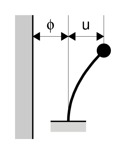
The equation of motion of the point mass on the ground is shown below.
In this case, the acceleration of the ground acts to the point mass.
\begin{equation}
m\cdot(\ddot{\phi}+\ddot{u})+c\cdot\dot{u}+k\cdot u=0
\end{equation}
In above, the acceleration of the point mass is equal to the total of the ground acceleration $\ddot{\phi}$ and the acceleration $\ddot{u}$ which is measured from the reference point in the structure.
The value of $\ddot{\phi}+\ddot{u}$ is called the absolute acceleration.
On the other hand, the damping force and the restoring force are expressed using $\dot{u}$ and $u$ which are measured from the reference point in the structure.
The values $\dot{u}$ and $u$ are called relative velocity and relative displacement, respectively.
The response spectrum is used for the understanding the characteristics of a earthquake motion.
And the response spectrum is expressed as a graph which indicates the relationship between the natural frequency of SDOF model and the maximum value of the absolute acceleration or relative velocity or the relative displacement.
Usially, following formula is used for the calculation of the response spectrum.
This can be obtained by dividing through by $m$ of original equation of motion and transposition of the ground acceleration $\ddot{\phi}$ .
\begin{equation}
\ddot{u}+2\cdot h\cdot\omega_0\cdot\dot{u}+\omega_0^2\cdot u=-\ddot{\phi}
\end{equation}
where, $h$ is damping factor of the system, $\omega_0$ is natural circular frequency of the system.
The relationships between $h$ , $\omega_0$ and $m$ , $c$ , $k$ are shown below.
\begin{equation}
c=2\cdot h\sqrt{k\cdot m} \qquad \omega_0=\sqrt{\cfrac{k}{m}} \qquad T=\cfrac{2\pi}{\omega_0}=2\pi\sqrt{\cfrac{m}{k}}
\end{equation}
where, $T$ is the natural period of the system.
In this section, we consider the program for calculation of the acceleration response spectrum for the earthquakemotion.
As a format of the equation of motion, we use following format taking into consideration of the use of dynamic analysis of a general structure.
Input datas are the ground acceleration by earthquake \ddot{\phi} , the damping factor $h$ and the natural period of system $T$ .
\begin{gather}
m\cdot\ddot{u}+c\cdot\dot{u}+k\cdot u=-m\cdot\ddot{\phi}\\
m=1 \qquad k=\frac{4\pi^2\cdot m}{T^2} \qquad c=2\cdot h \sqrt{k\cdot m}
\end{gather}
The basic setting in the program is shown below.
| Time interval of the ground acceleration record | $\Delta t$ (sec) |
| Calculation range of the natural period | $T=2\cdot\Delta t\sim 10$(sec) |
| Damping factor | $h=0.05$ |
Note that the maximum value of the absolute acceleration $\ddot{\phi}+\ddot{u}$ shall be searched and outputted as a acceleration response.
That is, since the relative acceleration $\ddot{u}$ is obtained as a solution of the equation of motion by the numerical integration,
it is necessary to get the absolute acceleration by adding the ground acceleration $\ddot{\phi}$ to the relative acceleration $\ddot{u}$ .
In the program, the equation of motion is solved using the linear acceleration method.
And the baseline correction of acceleration record is carried out using the subroutine by Dr.Ohsaki.
(Although the original subroutines are written using FORTRAN 77, these are rewritten into Fortran 90.)
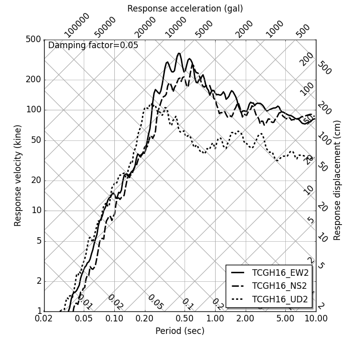
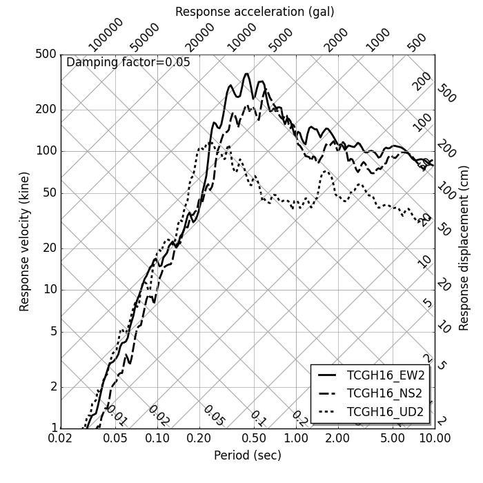
Tripartite response spectrum
In the graph of the tripartite response spectrum, the velocity response spectrum is drawn on the Log-Log plane firstly, next axes for acceleration and displacement response are appended.
By using this one, we can know the approxmate values of the acceleration, velocity and displacement from only one graph.
The axes for acceleration and displacement are defined using following relationships.
\begin{equation}
S_a\doteqdot\cfrac{2 \pi}{T}\cdot S_v \qquad\qquad S_d\doteqdot\cfrac{T}{2 \pi}\cdot S_v
\end{equation}
| where, | $S_a$ | : Maximum absolute acceleration response |
| | $S_v$ | : Maximum relative velocity response |
| | $S_d$ | : Maximum relative displacement response |
 |
 |
 |
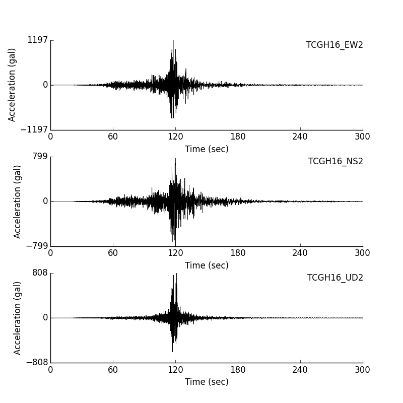
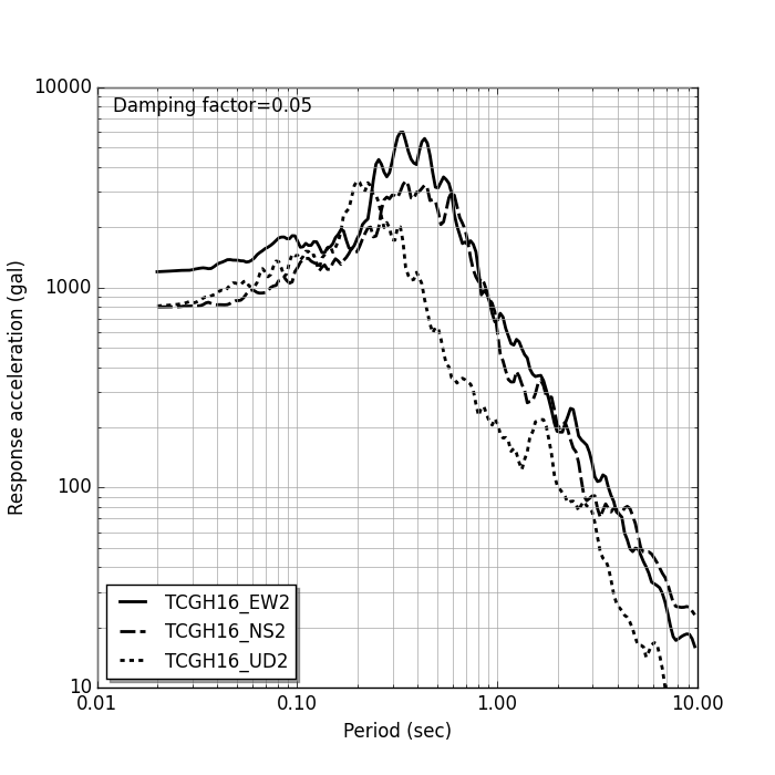
Input wave time history
(ground acceleration) |
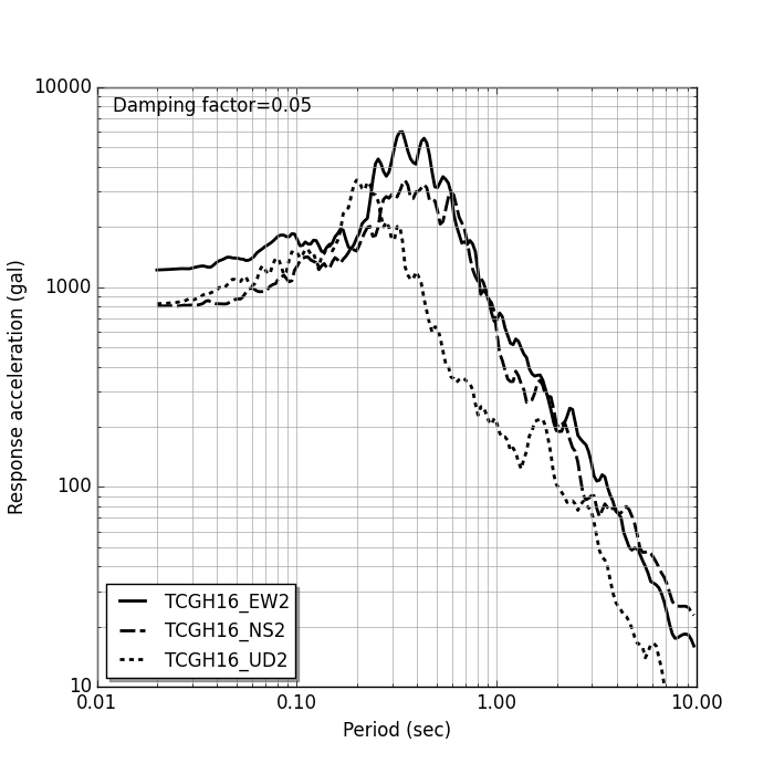
Acceleration response spectrum
by Linear acceleration method |
Tripartite response spectrum
by Linear acceleration method |
The source datas for sample calculations were downloaded from 'KiK-net' of National Research Institute for Earth Science and Disaster Prevention in Japan.
Inputted time history data of ground acceleration, the acceleration response spectrum and the tripartite response spectrum are shown above.
Fourier spectrum
Finite Fourier coefficient
Consider the following digital data.
| Sample number | $N$ |
| Time interval | $\Delta t$ |
| Digital value | $x_m \qquad m=0,1,2,\cdots,N-1$ |
Set the sample number $N=2^L$ ( $L$ : positive integer) as a value of a power of two in order to adopt the FFT.
And if we deem that $x_m$ can be expressed using the finite trigonometrical from $0$ to $N/2$ , following form can be obtained.
\begin{align}
x_m=&\sum_{k=0}^{N/2}\left\{A_k\cdot\cos\left(\frac{2\pi k}{N\cdot\Delta t}\cdot t\right)+B_k\cdot\sin\left(\frac{2\pi k}{N\cdot\Delta t}\cdot t\right)\right\} \\
=&\frac{A_0}{2}+\sum_{k=1}^{N/2-1}\left(A_k\cdot\cos\frac{2\pi k m}{N}+B_k\cdot\sin\frac{2\pi k m}{N}\right)+\frac{A_{n/2}}{2}\cdot\cos\frac{2\pi(N/2)m}{N}
\end{align}
\begin{equation}
m=0,1,2,\cdots,N-1 \qquad t=m\cdot\Delta t
\end{equation}
Above form is called the finite Fourier approximation of the function $x(t)$ , and $A_k, B_k$ are called the finite Fourier coefficients.
The mathematical operation to obtain the finite Fourier coefficients is called the Fourier transform.
The mathematical operation to obtain the digital sample data using known finite Fourier coefficients is called inverse Fourier transform.
\begin{align}
A_k=&\frac{2}{N}\sum_{m=0}^{N-1}x_m\cdot\cos\frac{2\pi k m}{N} & \qquad & k=0,1,2,\cdots,N/2-1,N/2 \\
B_k=&\frac{2}{N}\sum_{m=0}^{N-1}x_m\cdot\sin\frac{2\pi k m}{N} & \qquad & k=1,2,\cdots,N/2-1
\end{align}
\begin{equation}
\frac{A_0}{2}=\frac{1}{N}\sum_{m=0}^{N-1}x_m \qquad \text{(Average of all data)}
\end{equation}
Expression of finite Fourier transform in complex number
Express the Fourier transform and inverse Fourier transform in complex number using Euler's formula ( $e^{\pm i\theta}=\cos\theta \pm i\sin\theta$ ).
\begin{align*}
&\text{Fourier transform} &C_k=&\frac{1}{N}\sum_{m=0}^{N-1}x_m\cdot e^{-i(2\pi k m/N)} & k=&0,1,2,\cdots,N-1 \\
&\text{Inverse Fourier transform}&x_m=&\sum_{k=0}^{N-1}C_k\cdot e^{+i(2\pi k m/N)} & m=&0,1,2,\cdots,N-1
\end{align*}
Relationship between real Fourier coefficients and complex Fourier coefficients
\begin{equation*}
C_k=\frac{A_k-i B_k}{2} \qquad A_k+i B_k=A_{N-k}-i B_{N-k}
\end{equation*}
\begin{equation*}
A_k=2\cdot Re(C_k) \qquad B_k=-2\cdot Im(C_k) \qquad k=0,1,2,\cdots,N/2
\end{equation*}
Fourier amplitude spectrum and Fourier phase spectrum
\begin{align*}
&\text{Frequency} &~&f_k =\frac{k}{N\cdot\Delta t} \qquad k=0,1,2,\cdots,N/2 \\
&\text{Fourier amplitude}& &F_k =\frac{N\cdot\Delta t}{2}\sqrt{A_k{}^2+B_k{}^2}=N\cdot\Delta t|C_k|=N\cdot\Delta t\sqrt{Re(C_k)^2+Im(C_k)^2} \\
&\text{Phase angle} & &\phi_k =\arctan\left(-\frac{B_k}{A_k}\right)=\arctan\left(\frac{Im(C_k)}{Re(C_k)}\right) \qquad (-\pi<\phi_k<\pi) \\
&\text{Phase wave} & &\hat{x}(t)=\sum_{k=1}^{N/2}\cos(2\pi\cdot f_k \cdot t+\phi_k)
\end{align*}
The plots which shows the relationship between the frequencies and Fourier amplitudes are called the Fourier amplitude spectrum.
This can be called onlyFourier spectrum.
Simple use of Fourier transform and inverse Fourier transform
The results of use of Fourier transform and inverse Fourier transform are shown below.
- data was made using Fortran 90 subroutine 'random_number' with a sample number of 16.
- Re(Ck) and Im(Ck) are complex Fourier coefficients by Fast Fourier Transform.
- abs(Ck) is an absolute value of complex Fourier coefficients, and fp(k) is a phase angle.
- Re(xm) and Im(xm) are re-producted value using complex Fourier coefficients by inverse Fourier transform.
| i | data | Re(Ck) | Im(Ck) | abs(Ck) | fp(Ck) | Re(xm) | Im(xm) |
|---|
| 1 | 0.998 | 0.478 | 0.000 | 0.478 | 0.000 | 0.998 | 0.000 |
| 2 | 0.567 | 0.154 | -0.014 | 0.154 | -5.171 | 0.567 | 0.000 |
| 3 | 0.966 | -0.003 | -0.053 | 0.053 | -93.070 | 0.966 | 0.000 |
| 4 | 0.748 | -0.018 | -0.008 | 0.020 | -155.386 | 0.748 | 0.000 |
| 5 | 0.367 | 0.057 | -0.014 | 0.059 | -14.125 | 0.367 | 0.000 |
| 6 | 0.481 | 0.000 | 0.092 | 0.092 | 89.861 | 0.481 | 0.000 |
| 7 | 0.074 | 0.012 | 0.030 | 0.033 | 67.645 | 0.074 | 0.000 |
| 8 | 0.005 | 0.027 | -0.047 | 0.054 | -60.520 | 0.005 | 0.000 |
| 9 | 0.347 | 0.062 | 0.000 | 0.062 | 0.000 | 0.347 | 0.000 |
| 10 | 0.342 | 0.027 | 0.047 | 0.054 | 60.520 | 0.342 | 0.000 |
| 11 | 0.218 | 0.012 | -0.030 | 0.033 | -67.645 | 0.218 | 0.000 |
| 12 | 0.133 | 0.000 | -0.092 | 0.092 | -89.861 | 0.133 | 0.000 |
| 13 | 0.901 | 0.057 | 0.014 | 0.059 | 14.125 | 0.901 | 0.000 |
| 14 | 0.387 | -0.018 | 0.008 | 0.020 | 155.386 | 0.387 | 0.000 |
| 15 | 0.445 | -0.003 | 0.053 | 0.053 | 93.070 | 0.445 | 0.000 |
| 16 | 0.662 | 0.154 | 0.014 | 0.154 | 5.171 | 0.662 | 0.000 |
| Ave. | 0.478 | | | | | | |
From above table, we can know follows and they are expected results.
- Regarding the real parts of complex Fourier coefficients Re(Ck), 1st value for i=0 is equal to the average of all real data. And distribution of Re(Ck) is line symmetry to the point of $n/2+1$ st (i=8), where $n$ means sample number.
- Regarding the imaginary parts of complex Fourier coefficients Im(Ck), 1st value for i=0 is equal to zero. And distribution of Im(Ck) is point symmetry to the point of $n/2+1$ st (i=8), where $n$ means sample number.
- Regarding the result of inverse Fourier transform, the value of real parts Re(xm) are corresponded to inputted data, and all values of imaginary parts Im(xm) are deemed approxmately zero.
In this section, FFT program by Fortran 90 is used. This program was rewritten into Fortran 90 from BASIC program by Dr.Minami.
Note following items for use of this FFT program.
- For Fourier transform
Since this program outputs the part $\sum_{m=0}^{N-1}x_m\cdot e^{-i(2\pi k m/N)}$ in the expression $C_k=\frac{1}{N}\sum_{m=0}^{N-1}x_m\cdot e^{-i(2\pi k m/N)}$ ,
outputted data shall be divided by the sample number $N$ .
- For inverse Fourier transform
In order to obtain the value of acceleration from given complex Fourier coefficients by inverse Fourier transform,
the sign of imaginary parts of complex Fourier coefficients shall be reversed.
We can understand the necessity of this treatment by comparison of the exponential parts between the expression of complex Fourier coefficients.
Sample drawing of Fourier spectrum
Following relationships is drawn in the drawing of Fourier spectrum.
\begin{align*}
&\text{Frequency} &~&f_k=\frac{k}{N\cdot\Delta t} & (k=0\sim N/2)\\
&\text{Fourier amplitude}&~&F_k=N\cdot\Delta t\sqrt{Re(C_k)^2+Im(C_k)^2} & (k=0\sim N/2)
\end{align*}
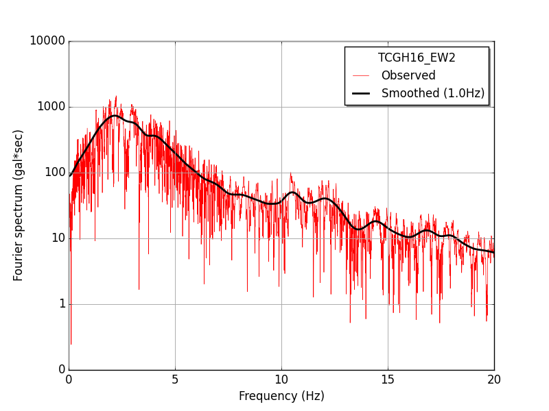
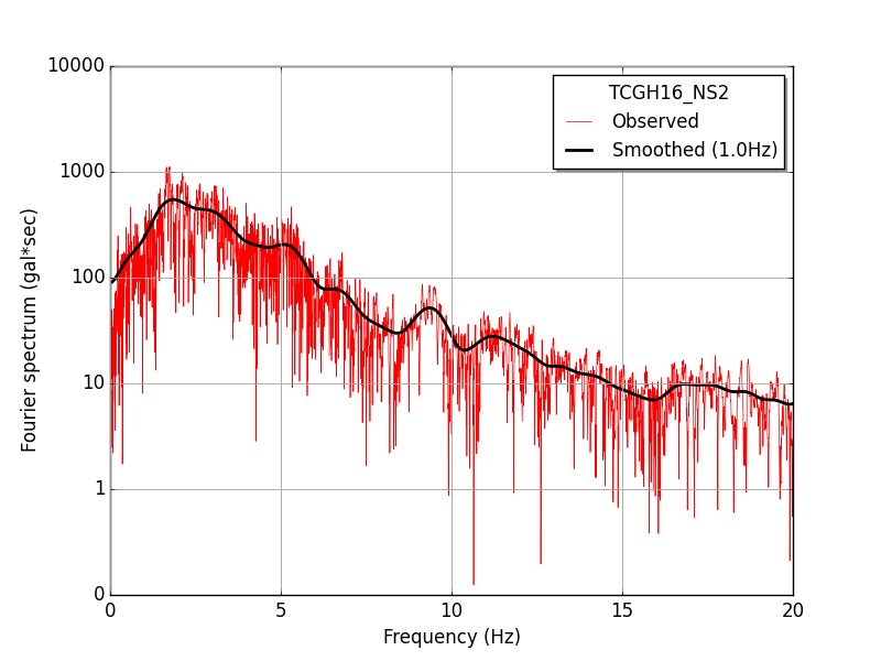
Fourier spectra for the ground acceleration shown in the figure of inputted time history data are indicated in following drawings.
In those drawings, black line means smoothed line by Parzen window with band width of 1.0Hz, and red line means non-smoothed results.
Used subroutine for Parzen window is rewritten into Fortran 90 from original subroutine 'SWIN' by Dr.Ohsaki.
 |
 |
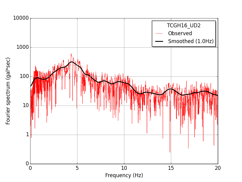 |
| Fourier spectrum (black line: after smoothing, red line: original) |
|---|
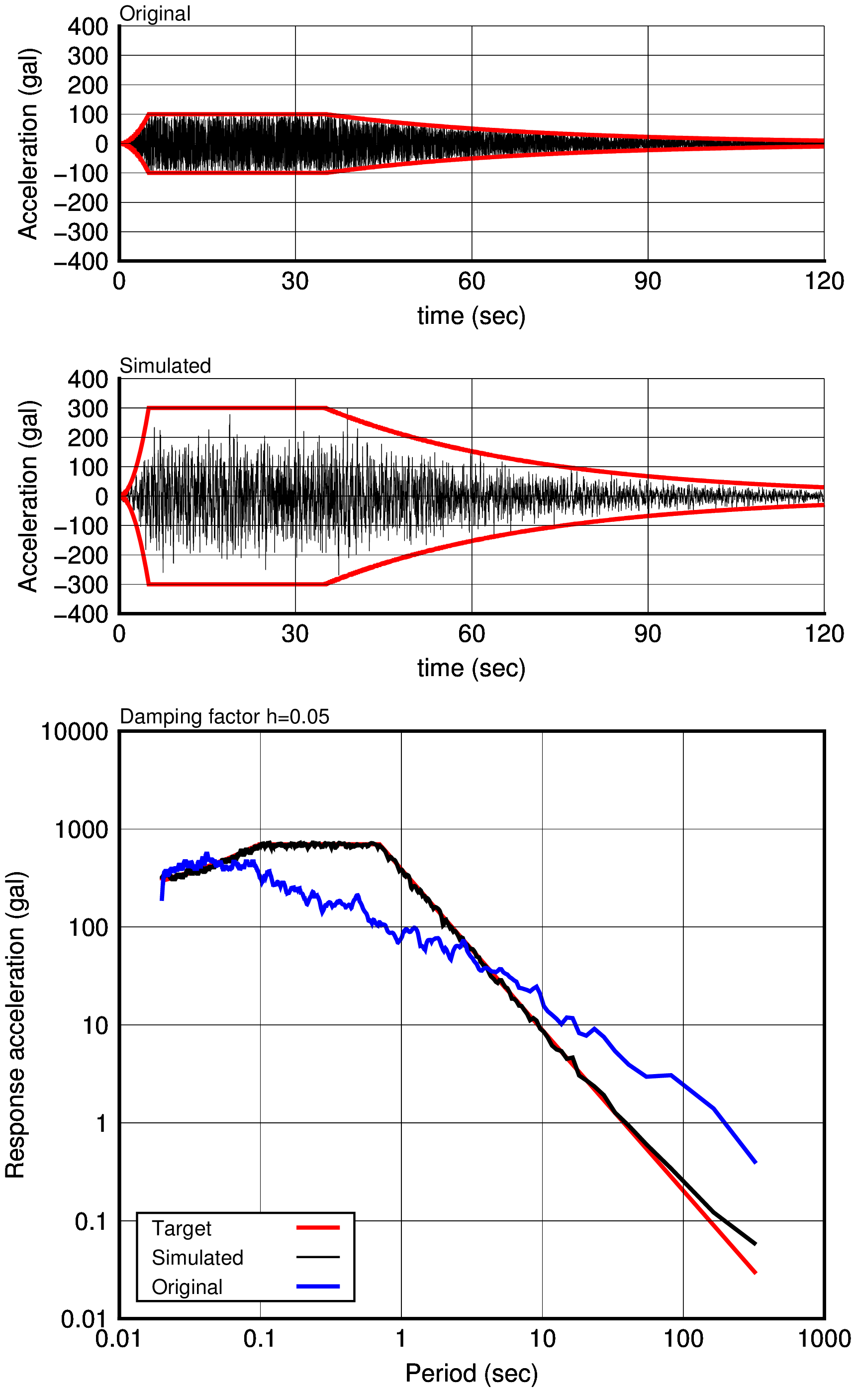
Simulated earthquake motion
Basic concept for making a simulated earthquake motion
- Basic concept of this method is reffered to 'Technical Note of National Institute for land and Infrastructure management, No.244, march 2005 (Guideline for the Seismic Performance Evaluation of dams against large earthquake (Draft))'.
- The target acceleration spectrum and initial wave (acceleration time history data) are required as input for this method.
And output is the acceleration time history data which fits the specified target spectrum.
- Allowable error for fitting is 5%. However, in case that error doesn't achieve the allowable value and error reaches the bottom, the iterative process is stopped.
- The time range of simulated earthquake motion is the same as it of inputted initial wave.
- Although the target spectrum is inputted as a function of the period, it is treated as a function of the frequency to adopt Fourier transform in the internal processing.
 |
| Process for making a simulated earthquake motion |
|---|
Effect of duration time of earthquake
Try to know the effect of duration time of earthquake using mentioned process. A Fortran program was made for this trial.
Duration time of earthquake was estimated using following thinking.
| Case considered | Envelope function |
|---|
| Case | a (sec) | b (sec) | c (sec) |
|---|
| 1 | 5 | 15 | 30 |
| 2 | 5 | 25 | 60 |
| 3 | 5 | 35 | 120 |
|
|
\begin{align*}
\begin{cases}
~~e(t)=(t/a)^2 \\
~~e(t)=1.0 \\
~~e(t)=\exp\{-\alpha\cdot(t-b)\} \qquad \alpha=-\cfrac{\ln(0.1)}{c-b} \\
~~e(t)=0.1 \qquad \text{at} \quad t=c
\end{cases}
\end{align*}
|
|
 |
| Envelop function |
|---|
Initial waves for this trial were made by following process.
- Obtain dataset of uniform random numbers with the range of $0\sim 1$ using the subroutine 'random_number' in Fortran 90.
- Enlarge the range of dataset to $-1\sim 1$, and obtain the initial wave by multipling enlarged dataset of random numbers by envelope function and specified maximum acceleration.
- Time interval is set to $\Delta t=0.01$ (sec).
- Maximum acceleration is set to 100gal.
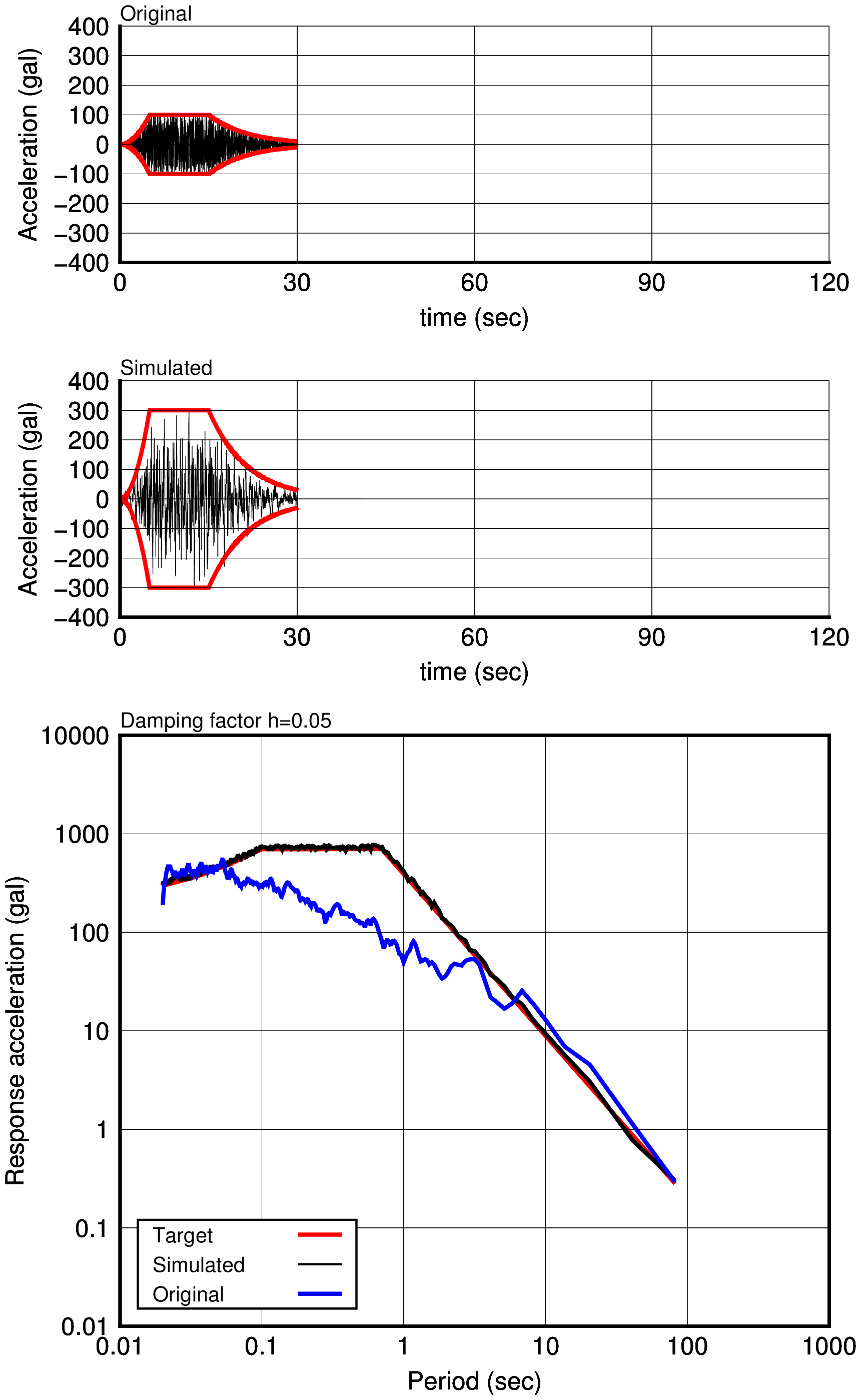
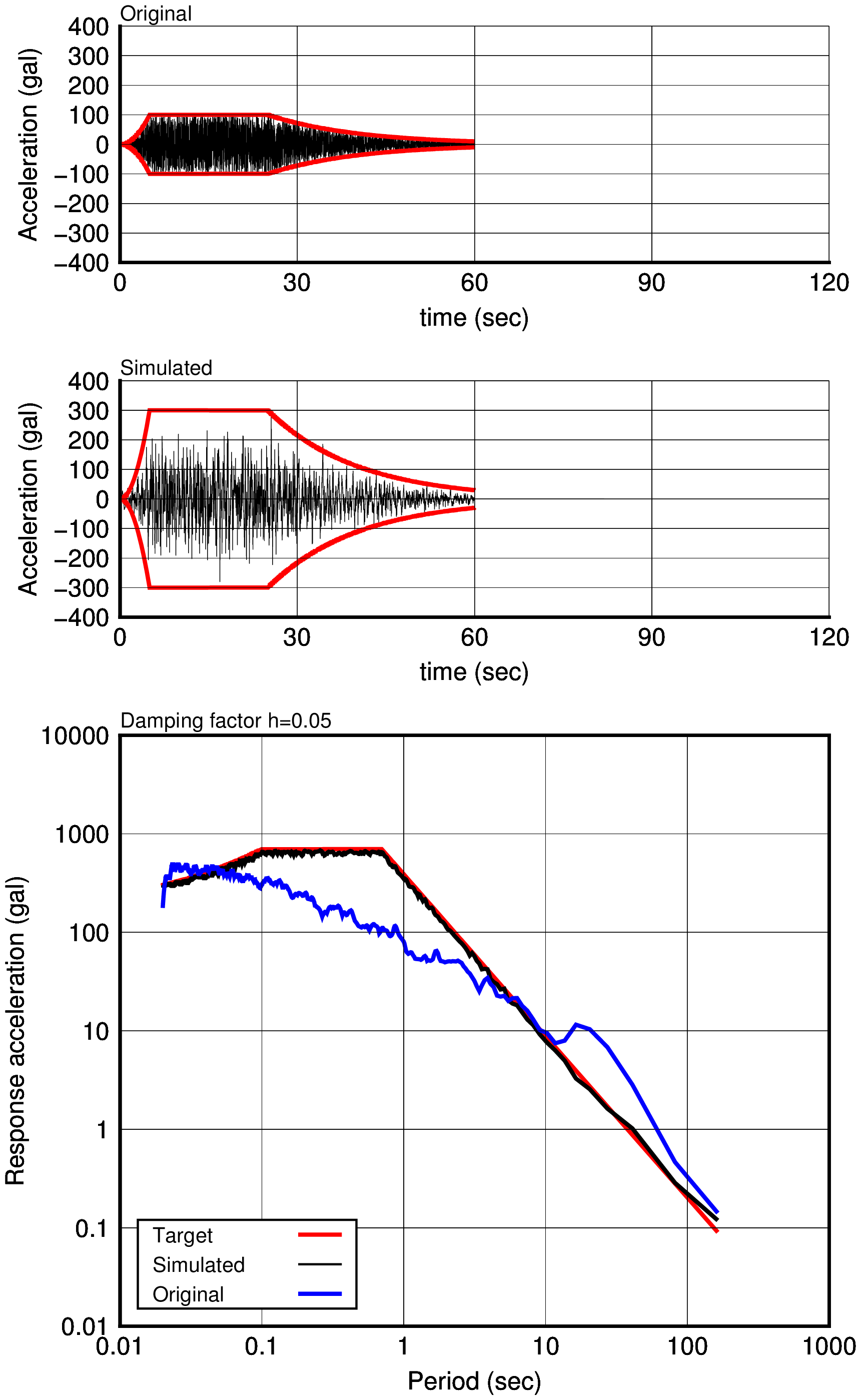
Some simulated earthquake motions were made using initial waves which were producted by above process.
maximum acceleration of target spectrum was set to 300gal.
Initial wave, simulated earthquake motion and acceleration response spectrum for each case are shown.
Please note that the purpose of these trial is only numerical testing, not practical work.
 |
 |
 |
| Case-1 (duration time c=30sec) |
Case-2 (duration time c=60sec) |
Case-3 (duration time c=120sec) |
Phase angle (sample using Case 1)
- The phase angles of initial wave are quite same as them of simulated earthquake motion.
- Above fact means that the phase angles of initial wave are maintained and Fourier amplitudes are changed to fit the target spectrum in used process.
- The shape of phase wave made from simulated earthquake motion is almost like it made from initial wave.
- Although the reason above can not be understood, it seems that the shape of phase wave of initial wave affects duration time and the shape of envelope function.

Fourier phase spectrum of input wave |

Input wave time history |

Fourier phase spectrum of simulated wave |

Simulated phase wave time history |
| Sample of Phase wave analysis |
|---|
Solution of equation of motion: Runge-Kutta method
calculation method
In order to apply Runge-Kutta method, it is becessary to convert the equation of motion to simultaneous differential equations shown below.
\begin{equation*}
\begin{cases}
\quad f_a(t,x,y)=\dot{x}=\cfrac{dx}{dt}=y \\
\quad \\
\quad f_b(t,x,y)=\ddot{x}=\cfrac{dy}{dt}=\cfrac{f(t)}{m}-\cfrac{c}{m}\cdot y-\cfrac{k}{m}\cdot x
\end{cases}
\end{equation*}
The simultaneous differential equations shown above can be solved applying Runge-Kutta method.
The procedure for Runge-Kutta method is shown below, where $h$ is a time increment of calculation.
Please take care to provide initial values for each variable of $t$ , $x$ and $y$ .
\begin{equation*}
\begin{cases}
&k_{a1}=f_a(t_n,x_n,y_n) \\
&k_{a2}=f_a(t_n+h/2,x_n+h/2\cdot k_{a1},y_n+h/2\cdot k_{a1}) \\
&k_{a3}=f_a(t_n+h/2,x_n+h/2\cdot k_{a2},y_n+h/2\cdot k_{a2}) \\
&k_{a4}=f_a(t_n+h,x_n+h\cdot k_{a3},y_n+h\cdot k_{a3}) \\
&x_{n+1}=x_n+h/6\cdot (k_{a1}+2k_{a2}+2k_{a3}+k_{a4})
\end{cases}
\end{equation*}
\begin{equation*}
\begin{cases}
&k_{b1}=f_b(t_n,x_n,y_n) \\
&k_{b2}=f_b(t_n+h/2,x_n+h/2\cdot k_{b1},y_n+h/2\cdot k_{b1}) \\
&k_{b3}=f_b(t_n+h/2,x_n+h/2\cdot k_{b2},y_n+h/2\cdot k_{b2}) \\
&k_{b4}=f_b(t_n+h,x_n+h\cdot k_{b3},y_n+h\cdot k_{b3}) \\
&y_{n+1}=y_n+h/6\cdot (k_{b1}+2k_{b2}+2k_{b3}+k_{b4})
\end{cases}
\end{equation*}
\begin{equation*}
\begin{cases}
\quad \ddot{x}=\cfrac{f(t)}{m}-\cfrac{c}{m}\cdot y_{n+1}-\cfrac{k}{m}\cdot x_{n+1} & \text{(acceleration)}\\
\quad \dot{x}=y_{n+1} & \text{(velocity)}\\
\quad x=x_{n+1} & \text{(displacement)}
\end{cases}
\end{equation*}
Stability of Runge-Kutta-method
We study the stability condition of Runge-Kutta method on the numerical integration of equation of motion.
For this purpose, we consider the simplest equation shown below.
\begin{equation}
\dot{z}=i\cdot\omega\cdot z
\end{equation}
Above equation is a differential equation related the velocity ( $\dot{z}$ ) and the displacement ( $z$ ) expressed in complex number,
and $\omega$ means natural angular frequency.
Adopt Runge-Kutta method to above differential equation.
\begin{align*}
k_1=&f(z_n) &=&i\omega z \\
k_2=&f(z_n+h/2\cdot k_1)&=&(i\omega-h/2\cdot\omega^2) z_n \\
k_3=&f(z_n+h/2\cdot k_2)&=&(i\omega-h/2\cdot\omega^2-i\cdot h^2/4\cdot\omega^3) z_n \\
k_4=&f(z_n+h \cdot k_2)&=&(i\omega-h \cdot\omega^2-i\cdot h^2/2\cdot\omega^3+h^3/4\cdot\omega^4) z_n
\end{align*}
\begin{align*}
z_{n+1}=&z_n+h/6 (k_1+2k_2+2k_3+k_4) \\
=&z_n\left\{1-\cfrac{1}{2}h^2\omega^2+\cfrac{1}{24}h^4\omega^4+i\left(h\omega-\cfrac{1}{6}h^3\omega^3\right)\right\}\\
=&z_n\left\{1-\cfrac{1}{2}x^2 +\cfrac{1}{24}x^4 +i\left(x -\cfrac{1}{6}x^3 \right)\right\}
\qquad \text{where, $x=h\omega$.}
\end{align*}
From above, following relationship can be obtained.
\begin{equation*}
\frac{z_{n+1}}{z_n}=\left\{1-\cfrac{1}{2}x^2+\cfrac{1}{24}x^4+i\left(x-\cfrac{1}{6}x^3\right)\right\}=A\cdot e^{i\theta}
\qquad \text{where, $x=h\omega$.}
\end{equation*}
The stability condition of this numerical integration is $|A|\leqq 1$ , and it can be expressed below.
\begin{equation*}
A^2=\left(1-\cfrac{1}{2}x^2+\cfrac{1}{24}x^4\right)^2+\left(x-\cfrac{1}{6}x^3\right)^2=1+\cfrac{x^6}{576}(x^2-8)\leqq 1
\end{equation*}
\begin{equation*}
x=h\omega\leqq 2\sqrt{2} \quad\Rightarrow\quad h\leqq\cfrac{2\sqrt{2}}{2\pi}T\doteqdot 0.450 T \qquad \text{where, $T$ is a natural period}
\end{equation*}
From above, if we want to know the behavior of the structure which has the natural period of 0.02 second,
the time increment for Runge-Kutta method shall be less than 0.009 second (0.02 $\times$ 0.45).
Calculation example
As a example of use of numerical integration of equation of motion, the calculation of the response spectrum for the earthquake wave acceleration was done using Runge-Kutta method.
Conditions for calculation of SDOF system is shown below.
\begin{equation*}
m=1 \qquad k=\frac{4\pi^2 m}{T^2} \qquad c=2h\sqrt{k m}
\end{equation*}
| Time interval of the ground acceleration record | $\Delta t=0.01$(sec) |
| Considered range of natural period of SDOF system | $T=0.02 \sim 10$(sec) |
| Damping factor | $h=0.05$ |
In addition, following things were considered for calculation.
- The interval of output is the same as input data interval (0.01sec).
- The interval of calculation by Runge-Kutta method is reduced to 1/5 (0.002sec) of the time interval of input data.
The interval of calculation shall be changed taking into consideration of the stability of numerical integration.
- Because, if the same time interval (0.01sec) as input data is used for calculation, the condition of stability can not be satisfied.
- The ground acceleration values are linearly interpolated for small time interval for calculation.
The results of calculation are shown below.
 |
 |
Acceleration response spectrum
by Runge-Kutta method |
Tripartite response spectrum
by Runge-Kutta method |
The source datas for sample calculations were downloaded from 'KiK-net' of National Research Institute for Earth Science and Disaster Prevention in Japan.
Solution of equation of motion: Frequency domain analysis for SDOF using FFT
As you know, there are two typical methods for numerical integration, one is a time domain analysis, and the ather is a frequency domain analisys using FFT.
In this section, frequency domain analysis for SDOF using FFT is introduced.
The equation of motion is shown below.
\begin{equation}
\ddot{u}(t)+2\cdot h\cdot\omega_0\cdot\dot{u}(t)+\omega_0^2\cdot u(t)=-a(t) \label{eq:frq1}
\end{equation}
where, $u$ is relative displacement of point mass, $a$ is acceleration of the ground, $h$ is damping factor of the system, $\omega_0$ is circular natural frequency of the system.
The acceleration of the ground, the displacement, velocity and acceleration of a point mass are expressed using inverse Fourier transform as follows.
\begin{align}
&a(t)=\frac{1}{2\pi}\int_{-\infty}^{\infty}A(\omega) e^{i\omega t}d\omega \\
&u(t)=\frac{1}{2\pi}\int_{-\infty}^{\infty}U(\omega) e^{i\omega t}d\omega \\
&\dot{u}(t)=\frac{1}{2\pi}\int_{-\infty}^{\infty}i\omega\cdot U(\omega) e^{i\omega t}d\omega \\
&\ddot{u}(t)=\frac{1}{2\pi}\int_{-\infty}^{\infty}-\omega^2\cdot U(\omega) e^{i\omega t}d\omega
\end{align}
Substituting above equations to the equation of motion, responses of displacement, velocity and acceleration can be obtained as follows.
\begin{align}
&U(\omega)=\frac{A(\omega)}{(\omega^2-\omega_0^2)-2 h \omega_0 \omega\cdot i} \\
&u(t)=\frac{1}{2\pi}\int_{-\infty}^{\infty}\frac{A(\omega)}{(\omega^2-\omega_0^2)-2 h \omega_0 \omega\cdot i} e^{i\omega t}d\omega \\
&\dot{u}(t)=\frac{1}{2\pi}\int_{-\infty}^{\infty}\frac{i\omega A(\omega)}{(\omega^2-\omega_0^2)-2 h \omega_0 \omega\cdot i} e^{i\omega t}d\omega \\
&\ddot{u}(t)=\frac{1}{2\pi}\int_{-\infty}^{\infty}\frac{-\omega^2 A(\omega)}{(\omega^2-\omega_0^2)-2 h \omega_0 \omega\cdot i} e^{i\omega t}d\omega
\end{align}
Where, following function $H(\omega)$ is called transfer function or frequency response function.
\begin{equation}
H(\omega)=\frac{1}{(\omega^2-\omega_0^2)-2 h \omega_0 \omega\cdot i}
\end{equation}
The process for calculation is shown below.
- Estimate complex Fourier coefficient $A(\omega)$ for inputted acceleration $a$ .
- Estimate transfer function $H(\omega)$ .
- Estimate time history of displacement $u(t)$ using IFFT for $A(\omega)\cdot H(\omega)$ .
- Estimate time history of velocity $\dot{u}(t)$ using IFFT for $i\omega\cdot A(\omega)\cdot H(\omega)$ .
- Estimate time history of acceleration $\ddot{u}(t)$ using IFFT for $-\omega^2\cdot A(\omega)\cdot H(\omega)$ .
Note following issues for using FFT.
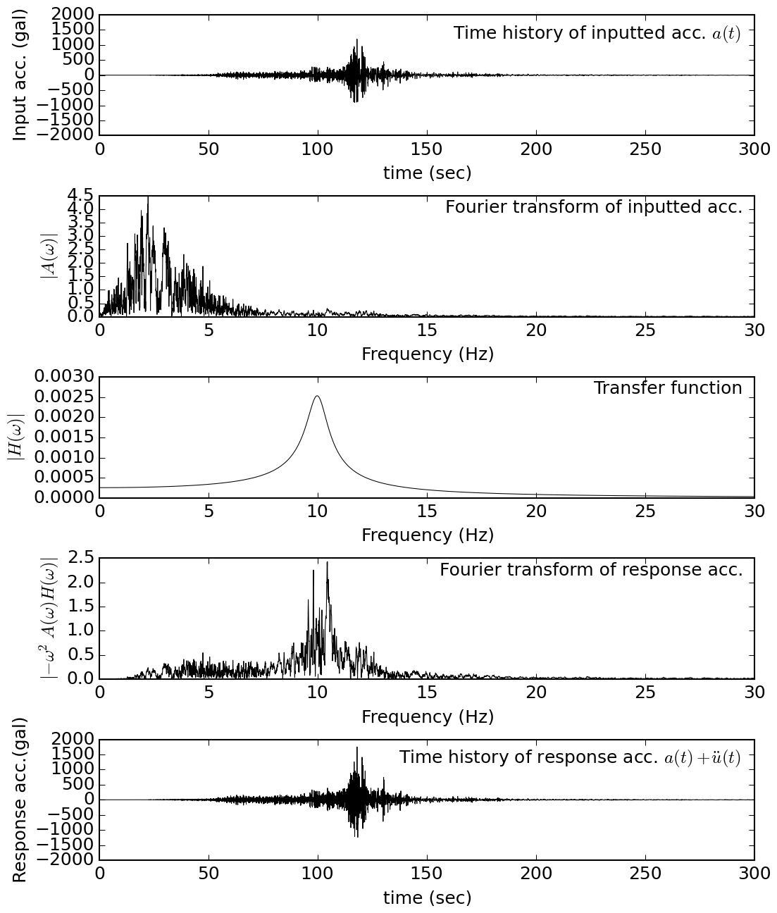 |
Steps for frequency domain analysis of SDOF (acceleration responce)
(damping factor: h=0.05, natural frequency: 10Hz) |
|---|
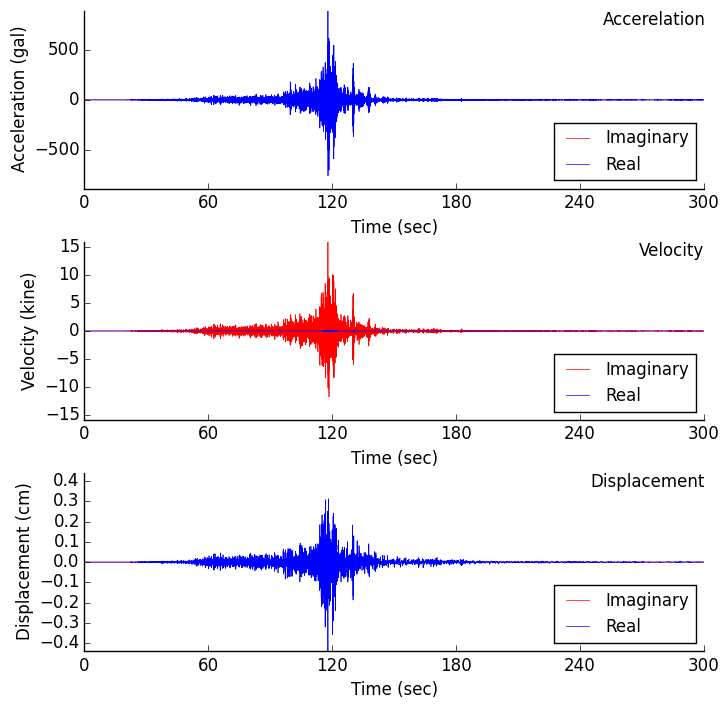 |
| Time histories of Acceleration, Velocity and Displacement |
|---|
In above drawings, the time histories of acceleration and displacement can be obtained as the values of real parts of IFFT results.
However, please note that the velocity response can be obtained as the value of imaginary part of IFFT result.
The response spectra which were calculated by this integration method are shown below.
 |
 |
Acceleration response spectrum
by FFT |
Tripartite response spectrum
by FFT |
The source datas for sample calculations were downloaded from 'KiK-net' of National Research Institute for Earth Science and Disaster Prevention in Japan.
Program source code
Solution of Motion of Equation, Response spectrum, Fourier spectrum
Simulated wave making